
Taylor Polynomials for Complex Functions: Mapping Diagrams
Loading the math board and drawing, please wait…
In collections
Mapping Diagrams to Visualize Complex Analysis
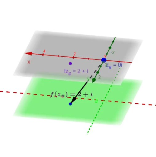
This example illustrates Taylor polynomials for complex functions and their mapping diagrams. Key mathematical concepts include complex functions, Taylor polynomials, and mapping diagrams. It utilizes commands like Sequence, Zip, Derivative, Sum, and If in GeoGebra. Suitable for university-level mathematics education and research.
GeoGebra Commands & Parameters
Sequence(0, n) → NZip(x^(nn), nn, N) → l3Derivative(F, z) → FzDerivative(Fz, z) → FzzDerivative(Fzz, z) → FzzzDerivative(Fzzz, z) → FzzzzSequence(0, m) → MZip(((2 * pi) * k / m), k, M) → t_*Zip((δ * ℯ^((t * ί))) + z_#, t, t_*) → z_*Zip(Simplify[Derivative[f, nn]] / nn!, nn, N) → l2Zip((xx(z) * yy(x)), xx, l2, yy, l3) → l4Sum(l4) → qIf(e ≟ 1, z_# - fz_#, 0) → alignCircle(z_#, δ) → cZip(f(z) + align, z, z_*) → fz_*Zip((x(z), y(z), ht), z, fz_*) → fpt_*Line(O, ZY1) → YaxLine(O, ZX1) → XaxZip(Vector[A, B], A, z_*, B, fpt_*) → fvec_*Vector(z_#, Fz1_#) → vecf_#Point(c) → A0Locus(PtAF, A0) → fLocIf(e ≟ 1, (x(z_#), y(z_#), ht), (x(fz_#), y(fz_#), ht)) → Alignfz_#Vector(z_#, Alignfz_#) → uTextfield(F) → InputBox1Locus(AF, A0) → loc1Zip((x(z), y(z)), z, fz_*) → l1Simplify(q(x, 0)) → TfTextfield(n) → InputBox2Zip(Tf(z) + align, z, z_*) → Tfz_*Zip((x(z), y(z), ht), z, Tfz_*) → Tfpt_*Zip(Vector[A, B], A, z_*, B, Tfpt_*) → Tfvec_*Locus(TFA3, A0) → TfLocSimplify(f(0) + (f'(0) * x) + (f''(0) / 2 * x^(2)) + (f'''(0) / 6 * x^(3)) + (f''''(0) / 24 * x^(4))) → TPfZip(TPf(z) + align, z, z_*) → TPfz_*Zip((x(z), y(z), ht), z, TPfz_*) → TPfpt_*Zip(Vector[A, B], A, z_*, B, TPfpt_*) → TPvec_*Locus(TPFA3, A0) → TPfLoc
AI Drawing Prompt Reference
Draw the Taylor polynomials of a complex function and their mapping diagrams. Start by plotting the complex function, then calculate its Taylor polynomial terms, and plot these polynomials to show their mapping relationships with the original function. Finally, display the local magnification of the Taylor polynomial and its approximation to the original function near the origin.
The prompt above was compiled from the original drawing commands and is for reference only.