
Systems of Inequalities 3
Loading the math board and drawing, please wait…
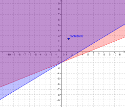
This example demonstrates the graphical representation of systems of inequalities. It involves key concepts such as inequalities and optimization. Using GeoGebra commands like DynamicCoordinates and Polygon, users can dynamically adjust parameters to observe changes in the graphical representation of the system. Suitable for high school mathematics education and learning.
GeoGebra Commands & Parameters
DynamicCoordinates(A, x(A), y(A)) → BDynamicCoordinates(A, x(A), y(A)) → CDynamicCoordinates(A, x(A), y(A)) → DDynamicCoordinates(A, x(A), y(A)) → EDynamicCoordinates(A, x(A), y(A)) → FDynamicCoordinates(A, x(A), y(A)) → GDynamicCoordinates(A, x(A), y(A)) → HDynamicCoordinates(A, x(A), y(A)) → IDynamicCoordinates(A, x(A), y(A)) → JDynamicCoordinates(A, x(A), y(A)) → KDynamicCoordinates(A, x(A), y(A)) → LDynamicCoordinates(A, x(A), y(A)) → MDynamicCoordinates(A, x(A), y(A)) → NDynamicCoordinates(A, x(A), y(A)) → ODynamicCoordinates(A, x(A), y(A)) → PPolygon(Q, R, 4) → poly1, q, r, s, t, S, TPolygon(Q_1, R_1, 4) → poly1_1, q_1, r_1, s_1, t_1, S_1, T_1