
Surface Area and Critical Points of the Octa-point Model's Functional Surface
Loading the math board and drawing, please wait…
In collections
₉Extreme Verteilung der 8 Punkten auf der Kugel
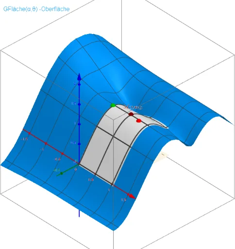
This example demonstrates the variation of the functional surface area of the octa-point model as parameters α and θ change. Core mathematical concepts include functions, derivatives, surface area, critical points, and optimization problems. It is constructed using GeoGebra commands/objects like Function, Derivative, Plane, Polygon, Textfield, and Point, as summarized. Suitable for high school students and math enthusiasts studying calculus, geometric constructions, and optimization problems.
GeoGebra Commands & Parameters
Function(GFläche(u, v), u, -1°, 60°, v, -1°, 90°) → mDerivative(GFläche(x, y), x) → GFläche_xDerivative(GFläche(x, y), y) → GFläche_yPlane(z = z0) → Plane0Polygon({(-1°, -1°), (60°, -1°), (60°, 90°), (-1°, 90°), (-1°, -1°)}) → Poly_{αθ}Textfield(Δθ) → InputBox1Point(xAxis) → Ca4Plane(z = 1.014575944622939) → Pl_{Lö2}Plane(z = 1) → Pl_{Lö1}
AI Drawing Prompt Reference
Draw a parametric surface showing how its surface area varies with parameters α and θ, defined over -1° to 60° and -1° to 90°, along with its two partial derivatives, and mark the critical points. Also, represent the parameter ranges of α and θ with a polygon on a plane, include an input box, and place a point on the x-axis.
The prompt above was compiled from the original drawing commands and is for reference only.