
Dancing Solution Curves of ODEs
Loading the math board and drawing, please wait…
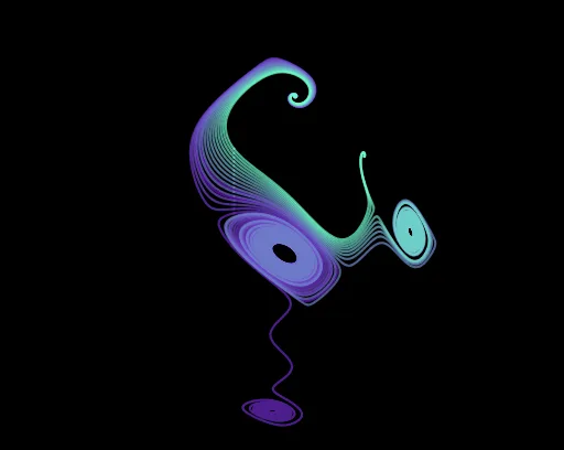
This example demonstrates the dynamic dancing effect of solution curves of ordinary differential equations (ODEs) as parameters vary. Key math concepts include ODEs, slope fields, solution curves, and parametric animation. Constructed using GeoGebra commands like SolveODE, SlopeField, t, f, button1, Ax, Ay, A, sol, n, speed, slp, and numerous objects A1-A18, B1-B11. Suitable for university students in mathematics or physics to study numerical solutions and visualizations of ODEs, or for educational demonstrations.
GeoGebra Commands & Parameters
SolveODE(f(x, y), Ax, Ay, 100, 0.08) → solSlopeField(f) → slpSolveODE(f(x, y), Ax, Ay + 0 - 0.8, 100, 0.08) → A1SolveODE(f(x, y), Ax, Ay + (13 / 170 * (2 - 1)) - 0.8, 100, 0.08) → A2SolveODE(f(x, y), Ax, Ay + (13 / 170 * (3 - 1)) - 0.8, 100, 0.08) → A3SolveODE(f(x, y), Ax, Ay + (13 / 170 * (4 - 1)) - 0.8, 100, 0.08) → A4SolveODE(f(x, y), Ax, Ay + (13 / 170 * (5 - 1)) - 0.8, 100, 0.08) → A5SolveODE(f(x, y), Ax, Ay + (13 / 170 * (6 - 1)) - 0.8, 100, 0.08) → A6SolveODE(f(x, y), Ax, Ay + (13 / 170 * (7 - 1)) - 0.8, 100, 0.08) → A7SolveODE(f(x, y), Ax, Ay + (13 / 170 * (8 - 1)) - 0.8, 100, 0.08) → A8SolveODE(f(x, y), Ax, Ay + (13 / 170 * (9 - 1)) - 0.8, 100, 0.08) → A9SolveODE(f(x, y), Ax, Ay + (13 / 170 * (10 - 1)) - 0.8, 100, 0.08) → A10SolveODE(f(x, y), Ax, Ay + (13 / 170 * (11 - 1)) - 0.8, 100, 0.08) → A11SolveODE(f(x, y), Ax, Ay + (13 / 170 * (12 - 1)) - 0.8, 100, 0.08) → A12SolveODE(f(x, y), Ax, Ay + (13 / 170 * (13 - 1)) - 0.8, 100, 0.08) → A13SolveODE(f(x, y), Ax, Ay + (13 / 170 * (14 - 1)) - 0.8, 100, 0.08) → A14SolveODE(f(x, y), Ax, Ay + (13 / 170 * (15 - 1)) - 0.8, 100, 0.08) → A15SolveODE(f(x, y), Ax, Ay + (13 / 170 * (16 - 1)) - 0.8, 100, 0.08) → A16SolveODE(f(x, y), Ax, Ay + (13 / 170 * (17 - 1)) - 0.8, 100, 0.08) → A17SolveODE(f(x, y), Ax, Ay + (13 / 170 * (18 - 1)) - 0.8, 100, 0.08) → A18SolveODE(f(x, y), Ax, Ay + 0 - 0.8, -100, 0.08) → B1SolveODE(f(x, y), Ax, Ay + (13 / 170 * (2 - 1)) - 0.8, -100, 0.08) → B2SolveODE(f(x, y), Ax, Ay + (13 / 170 * (3 - 1)) - 0.8, -100, 0.08) → B3SolveODE(f(x, y), Ax, Ay + (13 / 170 * (4 - 1)) - 0.8, -100, 0.08) → B4SolveODE(f(x, y), Ax, Ay + (13 / 170 * (5 - 1)) - 0.8, -100, 0.08) → B5SolveODE(f(x, y), Ax, Ay + (13 / 170 * (6 - 1)) - 0.8, -100, 0.08) → B6SolveODE(f(x, y), Ax, Ay + (13 / 170 * (7 - 1)) - 0.8, -100, 0.08) → B7SolveODE(f(x, y), Ax, Ay + (13 / 170 * (8 - 1)) - 0.8, -100, 0.08) → B8SolveODE(f(x, y), Ax, Ay + (13 / 170 * (9 - 1)) - 0.8, -100, 0.08) → B9SolveODE(f(x, y), Ax, Ay + (13 / 170 * (10 - 1)) - 0.8, -100, 0.08) → B10SolveODE(f(x, y), Ax, Ay + (13 / 170 * (11 - 1)) - 0.8, -100, 0.08) → B11SolveODE(f(x, y), Ax, Ay + (13 / 170 * (12 - 1)) - 0.8, -100, 0.08) → B12SolveODE(f(x, y), Ax, Ay + (13 / 170 * (13 - 1)) - 0.8, -100, 0.08) → B13SolveODE(f(x, y), Ax, Ay + (13 / 170 * (14 - 1)) - 0.8, -100, 0.08) → B14SolveODE(f(x, y), Ax, Ay + (13 / 170 * (15 - 1)) - 0.8, -100, 0.08) → B15SolveODE(f(x, y), Ax, Ay + (13 / 170 * (16 - 1)) - 0.8, -100, 0.08) → B16SolveODE(f(x, y), Ax, Ay + (13 / 170 * (17 - 1)) - 0.8, -100, 0.08) → B17SolveODE(f(x, y), Ax, Ay + (13 / 170 * (18 - 1)) - 0.8, -100, 0.08) → B18
AI Drawing Prompt Reference
Draw a set of solution curves for ordinary differential equations to demonstrate their dynamic dancing effect as parameters vary. Start by plotting the base solution curve, then generate multiple solution curves based on it, adjusting the slope parameters to make them dynamically change around the base curve, creating a dancing effect. Also display the slope field as a background to help understand the dynamic variation of the solution curves.
The prompt above was compiled from the original drawing commands and is for reference only.