Stable/Unstable Equilibrium Solutions Visualization

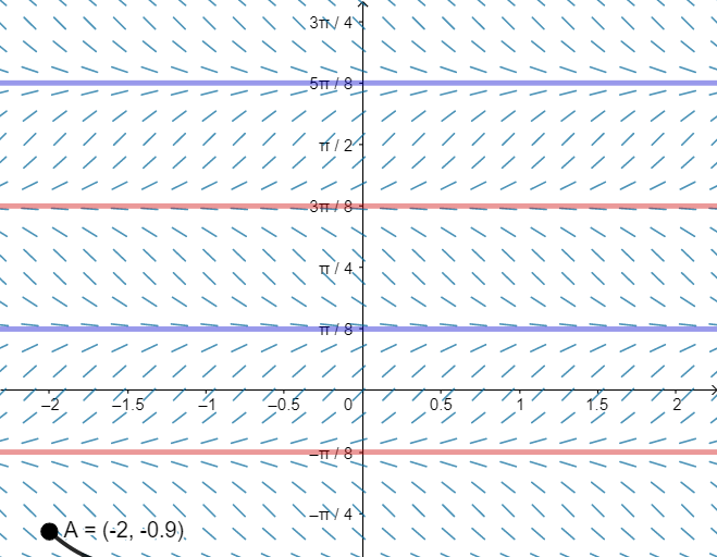
This GeoGebra example demonstrates stable and unstable equilibrium solutions of a first-order differential equation using slope fields and numerical solving. The core mathematical concept is the stability of equilibrium points: a stable equilibrium attracts nearby solution curves, while an unstable one repels them. The construction employs the SlopeField command to render the direction field, and SolveODE to compute particular solutions from initial conditions. Interactive elements include a button (button1) and a slider (a) to adjust parameters, allowing users to observe how the equilibrium position and its stability change. Objects such as A, f, F, Sol1, g, h, i, j define functions, solution curves, and auxiliary graphics. This resource is ideal for university-level differential equations courses or advanced high school mathematics, providing a visual and hands-on approach to understanding equilibrium stability and the use of computational tools in dynamical systems analysis.