
Squirrel's Acorn Stash: One Side of a Linear Equation by George Gardner
Loading the math board and drawing, please wait…
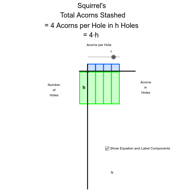
This example uses digital algebra tiles to help students find a part of the solution to a linear equation problem. It demonstrates how to solve real-world problems using linear equations. Key mathematical concepts include linear equations. Using GeoGebra commands such as Intersect, Point, and Polygon, students can visually understand the solution to a linear equation. Suitable for middle school mathematics education.
GeoGebra Commands & Parameters
Intersect(xAxis, yAxis) → APoint(xAxis) → BPoint(yAxis) → DPolygon(A, B, C, D) → poly1, a, b, c, dPoint(yAxis) → EVector(E, F) → uTranslate(A, u) → A'Translate(B, u) → B'Translate(C, u) → C'Translate(D, u) → D'Polygon(A', B', C', D') → poly1', a', b', c', d'Translate(A', u) → A''Translate(B', u) → B''Translate(C', u) → C''Translate(D', u) → D''Polygon(A'', B'', C'', D'') → poly1'', a'', b'', c'', d''Translate(A'', u) → A'''Translate(B'', u) → B'''Translate(C'', u) → C'''Translate(D'', u) → D'''Polygon(A''', B''', C''', D''') → poly1''', a''', b''', c''', d'''Translate(A''', v) → GTranslate(B''', v) → HTranslate(C''', v) → ITranslate(D''', v) → JTranslate(A''', u) → KTranslate(B''', u) → LTranslate(C''', u) → MTranslate(D''', u) → NPolygon(K, L, M, N) → poly2, k, l, m, nSequence(Polygon[(0, (-i)), (-1, (-i)), (-1, (-i) + 4), (0, (-i) + 4)], i, 4, (4 * num2), 4) → list2Sequence(Polygon[(0, ((-4) * num2) - j), (0, ((-4) * num2) - (j - 1)), 4], j, 1, con2, 1) → list3Sequence(Polygon[((4 * num) + j - 1, 0), ((4 * num) + j, 0), 4], j, 1, con1, 1) → list4Sequence(Sequence[Polygon[((4 * (n - 1)), ((-4) * m)), ((4 * n), ((-4) * m)), 4], m, 1, num2], n, 1, num) → list1Segment(P, Q) → eSegment(R, S) → fSequence(Sequence[Polygon[((4 * i), ((-4) * num2) - j), ((4 * i), ((-4) * num2) - j + 1), ((4 * (i - 1)), ((-4) * num2) - j + 1), ((4 * (i - 1)), ((-4) * num2) - j)], j, 1, con2], i, 1, num) → list6Sequence(Sequence[Polygon[((4 * num) + j - 1, ((-4) * (i - 1))), ((4 * num) + j, ((-4) * (i - 1))), ((4 * num) + j, ((-4) * i)), ((4 * num) + j - 1, ((-4) * i))], j, 1, con1], i, 1, num2) → list7Sequence(Sequence[Polygon[((4 * num) + j - 1, ((-4) * num2) - i), ((4 * num) + j, ((-4) * num2) - i), 4], j, 1, con1], i, 1, con2) → list5Polygon(T, U, V, W) → poly3, t, u_1, v_1, wPolygon(D_1, E_1, F_1, G_1) → poly5, d_1, e_1, f_1, g_1
AI Drawing Prompt Reference
Draw a coordinate system with the x-axis and y-axis intersecting at the origin. Take point B on the x-axis and point D on the y-axis, and use these four points to draw a rectangle. Then, translate this rectangle along the y-axis to form a series of parallel rectangles. Next, draw two line segments e and f from the origin, passing through these rectangles. Finally, draw a region containing these rectangles and another parallel region to form a shape for illustrating the solution to a linear equation.
The prompt above was compiled from the original drawing commands and is for reference only.