
Square Root Spiral: Geometric Construction and Dynamic Visualization
Loading the math board and drawing, please wait…
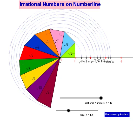
① This example demonstrates the construction of the Square Root Spiral (Spiral of Theodorus) by sequentially building right triangles, visualizing irrational numbers geometrically. ② Core mathematical concepts include square roots, right triangles, the Pythagorean theorem, irrational numbers on the real line, and iterative geometric construction. ③ Construction details: Using GeoGebra commands such as Intersect, Circle, Segment, OrthogonalLine, Line, CircleArc, Angle, Polygon, Centroid, Midpoint, and Ray, the spiral is formed by repeatedly creating right triangles with one leg of length 1, so that successive hypotenuses have lengths √2, √3, √4, etc., producing a spiral chain. ④ Suitable for middle and high school students to explore the connection between irrational numbers, the Pythagorean theorem, and geometric construction, and can serve as a hands-on math experiment or inquiry-based learning activity.
GeoGebra Commands & Parameters
Intersect(xAxis, yAxis) → ACircle(B, a) → cSegment(A, B) → fOrthogonalLine(B, f) → gIntersect(c, g) → C, DSegment(A, D) → hCircle(D, a) → dOrthogonalLine(D, h) → iIntersect(d, i) → E, FSegment(A, F) → jCircle(F, a) → eOrthogonalLine(F, j) → kIntersect(e, k) → G, HSegment(A, H) → lCircle(H, a) → pOrthogonalLine(H, l) → mIntersect(p, m) → I, JSegment(J, A) → nOrthogonalLine(J, n) → qCircle(J, a) → rIntersect(r, q) → K, LSegment(K, A) → sCircle(K, a) → tOrthogonalLine(K, s) → bIntersect(t, b) → M, NSegment(M, A) → f_1Circle(M, a) → c_1OrthogonalLine(M, f_1) → g_1Intersect(c_1, g_1) → O, PSegment(O, A) → h_1Circle(O, a) → d_1OrthogonalLine(O, h_1) → i_1Intersect(d_1, i_1) → Q, RSegment(Q, A) → j_1Circle(Q, a) → e_1OrthogonalLine(Q, j_1) → k_1Intersect(e_1, k_1) → S, TSegment(S, A) → l_1Circle(S, a) → p_1OrthogonalLine(S, l_1) → m_1Intersect(p_1, m_1) → U, VSegment(U, A) → n_1Line(A, B) → q_1Circle(A, D) → r_1Circle(A, F) → s_1Circle(A, H) → t_1Circle(A, J) → c_2Circle(A, K) → d_2Circle(A, M) → e_2Circle(A, O) → f_2Circle(A, Q) → g_2Circle(A, S) → h_2Circle(A, U) → k_2Intersect(k_2, q_1) → W, ZIntersect(h_2, q_1) → A_1, B_1Intersect(g_2, q_1) → C_1, D_1Intersect(f_2, q_1) → E_1, F_1Intersect(e_2, q_1) → G_1, H_1Intersect(d_2, q_1) → I_1, J_1Intersect(c_2, q_1) → K_1, L_1Intersect(t_1, q_1) → M_1, N_1Intersect(s_1, q_1) → O_1, P_1Intersect(r_1, q_1) → Q_1, R_1CircleArc(A, R_1, D) → p_2CircleArc(A, P_1, F) → q_2CircleArc(A, N_1, H) → r_2CircleArc(A, L_1, J) → s_2CircleArc(A, J_1, K) → t_2CircleArc(A, H_1, M) → c_3CircleArc(A, F_1, O) → d_3CircleArc(A, D_1, Q) → e_3CircleArc(A, B_1, S) → f_3CircleArc(A, Z, U) → g_3Segment(D, B) → a_1Segment(F, D) → b_1Segment(H, F) → i_2Segment(J, H) → j_2Segment(K, J) → l_2Segment(M, K) → m_2Segment(O, M) → n_2Segment(Q, O) → a_2Segment(S, Q) → b_2Segment(U, S) → h_3Angle(D, B, A) → αAngle(F, D, A) → βAngle(H, F, A) → γAngle(J, H, A) → δAngle(K, J, A) → εAngle(M, K, A) → ζAngle(O, M, A) → ηAngle(Q, O, A) → θAngle(S, Q, A) → ιAngle(U, S, A) → κPolygon(A, B, D) → t1, d_4, a_3, b_3Polygon(A, D, F) → t2, f_4, a_4, d_5Polygon(A, F, H) → t3, h_4, a_5, f_5Polygon(A, H, J) → t4, j_3, a_6, h_5Polygon(A, J, K) → t5, k_3, a_7, j_4Polygon(A, K, M) → t6, m_3, a_8, k_4Polygon(A, M, O) → t7, o, a_9, m_4Polygon(A, O, Q) → t8, q_3, a_{10}, o_1Polygon(A, Q, S) → t9, s_3, a_{11}, q_4Polygon(A, S, U) → t10, u, a_{12}, s_4Centroid(t1) → S_1Centroid(t2) → T_1Centroid(t3) → U_1Centroid(t4) → V_1Centroid(t5) → W_1Centroid(t6) → Z_1Midpoint(n_2) → A_2Centroid(t7) → B_2Centroid(t8) → C_2Centroid(t9) → D_2Centroid(t10) → E_2Ray(A, B) → i_3
AI Drawing Prompt Reference
In a Cartesian coordinate plane, use the intersection of the x-axis and y-axis as the starting point. First draw a segment from the start to a point on the x-axis, then construct a circle centered at that endpoint with the segment length as radius. Through the same endpoint, draw a perpendicular line to form another intersection with the circle, and connect the start point to the appropriate intersection to obtain the first right triangle’s hypotenuse. Repeat the process iteratively: at the newest endpoint, draw a circle with radius equal to the current segment to the start, draw the perpendicular line to create the next intersection points, and connect the start to the chosen intersection. This creates a chain of consecutive right triangles whose hypotenuse lengths increase like √2, √3, √4, … forming the geometric square-root spiral.
The prompt above was compiled from the original drawing commands and is for reference only.