Solving Linear Equations of the Form ax + b = c

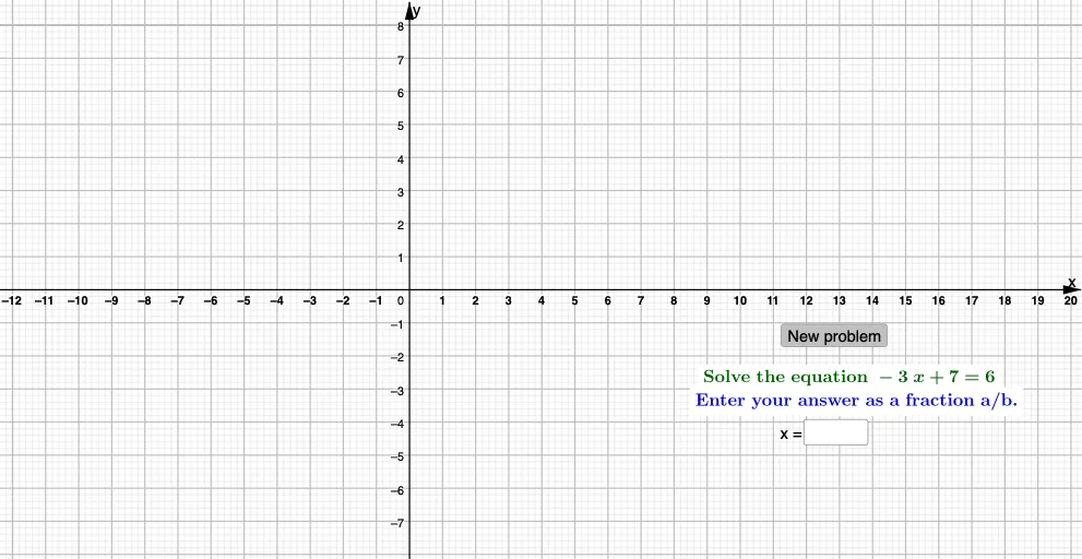
This GeoGebra example demonstrates how to solve linear equations of the type ax + b = c interactively. It visualizes the solution process by graphing the linear function and using the intersection of lines, while allowing users to adjust parameters a, b, and c via sliders or random generation. Core concepts include solving linear equations, function graphs, parametric modeling, and graphical solution methods. The construction uses GeoGebra commands such as Random, Intersect, Textfield, If, and Point to dynamically display the solution and provide an input box for verification. It is designed for high school algebra and introductory function courses, serving as an effective interactive tool for exploring linear equations.