
Solving 1-Step Subtraction Equations
Loading the math board and drawing, please wait…
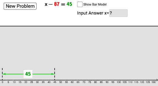
This example demonstrates solving 1-step subtraction equations. Key mathematical concepts include equation solving. Using GeoGebra commands such as Intersect, Random, Polygon, etc., the solution process is dynamically illustrated. Suitable for middle school mathematics education.
GeoGebra Commands & Parameters
Intersect(f, xAxis) → ARandom(0, 50) → aIntersect(g, xAxis) → CIntersect(h, xAxis) → BPolygon(G, I, S, R) → poly1, q, r, s, tPolygon(E, F, I, H) → poly2, e_1, f_1, i, h_2Min(-2, b - 2) → xMinSegment(E, B) → cSegment(I, C) → kMidpoint(c) → MMidpoint(F, C) → NSegment(D, A) → lMidpoint(l) → PMidpoint(P, M) → QMidpoint(R, G) → TMidpoint(S, I) → UMidpoint(T, U) → VPolygon(W, A_1, B_1, Z) → poly3, w_1, a_1, b_1, z_1Midpoint(P, A) → C_1Midpoint(P, D) → D_1Midpoint(M, B) → F_1Midpoint(N, C) → G_1Midpoint(N, F) → H_1Midpoint(C_1, F_1) → OTextfield(j) → InputBox1Midpoint(M, E) → I_1Midpoint(D_1, I_1) → J_1Max(2, a + b + 2) → xMaxSequence(Segment[D + (n * (1, 0)), G + (n * (1, 0))], n, 1, a, 1) → list1Polygon(D, E, H, G) → poly4, d, e, h_1, g_1Midpoint(C_1, G_1) → KMidpoint(L, R) → L_1Midpoint(K_1, S) → M_1Midpoint(M_1, L_1) → N_1Vector(L_1, M_1) → wIntersect(r, s) → P_1Segment(P_1, K_1) → j_1Vector(P, M) → mVector(M, P) → nVector(M, N) → uMidpoint(M, N) → JSegment(L, R) → i_1Sequence(Segment[E + (n * (1, 0)), H + (n * (1, 0))], n, 1, b, 1) → list2If(j ≟ a + b, "Correct!", If[j ≟ a - b ∨ j ≟ (-(b + a)) ∨ j ≟ (-(a - b)), "Check your sign/operation", "Incorrect..."]) → text1
AI Drawing Prompt Reference
Draw a dynamic illustration showing the solution of one-step subtraction equations. Include intersections of two lines with the x-axis, randomly generated values, and use polygons and line segments to demonstrate the equation-solving process. Display an equation input box and answer judgment, along with multiple midpoints and vector relationships, ultimately presenting a geometric solution approach.
The prompt above was compiled from the original drawing commands and is for reference only.