
Solids of Revolution (Parts 2 & 3) – Cones, Logarithms, and Incircles
Loading the math board and drawing, please wait…
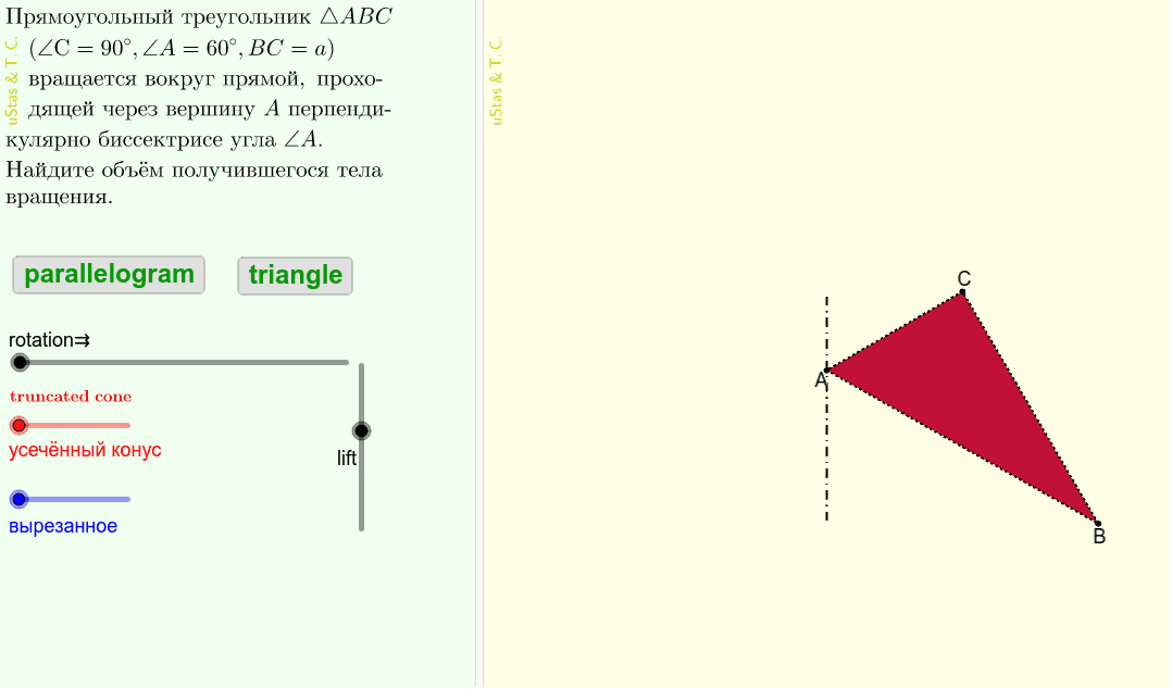
This GeoGebra example demonstrates the dynamic construction of solids of revolution, focusing on cones, logarithmic curves, and incircles. It visualizes how rotating 2D shapes around an axis generates 3D solids, integrating concepts such as volume of revolution, cone geometry, logarithmic functions, tangent and incircle properties, along with frequency distribution and exponential behavior. The construction uses commands like RotateText, Surface, Cone, Polygon, and Segment, with button scripts that redefine objects to animate the revolution. Suitable for high school to undergraduate students studying solid geometry, introductory calculus, and dynamic mathematics, this file aids in intuitively grasping the relationships between 2D profiles and their 3D rotational counterparts.
GeoGebra Commands & Parameters
RotateText("uStas\;\&\,Т.С.", 90°) → надпись01Surface((j * sin(i)), (j * cos(i)), zQ + ut + (((-1)^(L5) * k3) * (R - j)), i, 0, λ, j, r, R) → ηCone(U, Q, RR) → φ, ω, ΦCone(T, Q, (2 * m)) → ψ, Ω, ΠPolygon(Q, B', C') → s7, c', q, b'Polygon(Q, B', C', D') → s5, q_1, b'_1, c'_1, d'Segment(U + (0, 0, m), Q + (0, 0, (-m))) → d5Segment(U, T) → d7Segment(B, C) → aSegment(B', C') → cSegment(Q, B) → fSegment(Q, C) → eSegment(C, D) → kSegment(D, Q) → l