
Solids of Revolution - Disk Integration - Exploration & Practice
Loading the math board and drawing, please wait…
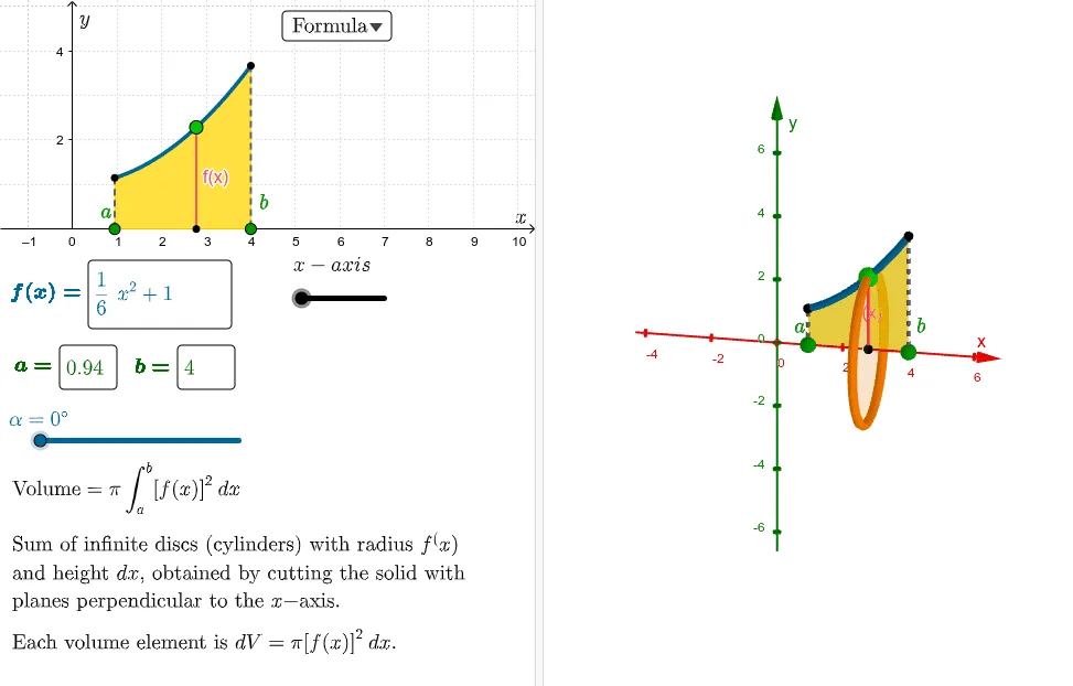
① This interactive GeoGebra example demonstrates how a plane curve rotated around an axis forms a solid of revolution, and computes its volume using the disk integration method. ② Core mathematical concepts include definite integrals, volume of revolution, function graphing, and 3D surfaces, with dynamic parameter control. ③ Construction highlights: Surface command generates the 3D rotated surface, Integral/IntegralBetween compute the definite integral, Rotate performs the rotation, Textfield and sliders (CampoInserimento) allow user input, while Point, Segment, Circle, and SelectedIndex support interactive exploration and switching between functions. ④ Suitable for high school to college calculus courses, especially for visualizing the derivation of the volume formula and for hands-on practice exploring how different functions affect the resulting volume.
GeoGebra Commands & Parameters
Textfield(f) → CampoInserimento1Textfield(a) → CampoInserimento2Textfield(b) → CampoInserimento3Point(g) → ASegment(AX, A) → hSegment(D, B) → iSegment(E, C) → jSurface(t, (g(t) * cos(u)), (g(t) * sin(u)), t, a, b, u, 0, α) → SupXIntegral(f, a, b) → intSurface(t, (u * f(t)), 0, t, a, b, u, 0, 1) → Integr3DRotate(Integr3D, α, xAxis) → Integr3D'CurveCartesian(t, (f(t) * cos(α)), (f(t) * sin(α)), t, a, b) → RotXRotate(A, α, xAxis) → A'Rotate(E, α, xAxis) → E'Rotate(D, α, xAxis) → D'CurveCartesian(x(C), y(C) + (y(E) * cos(t)), z(C) + (y(E) * sin(t)), t, 0, α) → Cfr2xCurveCartesian(x(B), y(B) + (y(D) * cos(t)), z(B) + (y(D) * sin(t)), t, 0, α) → Cfr1xSelectedIndex(scelte) → isSegment(AY, A) → nRotate(Integr3D, (-α), yAxis) → Integr3D'_1CurveCartesian((x(B) * cos(t)), 0, (x(B) * sin(t)), t, 0, α) → cCurveCartesian((x(C) * cos(t)), 0, (x(C) * sin(t)), t, 0, α) → eCurveCartesian((a * cos(t)), y(D), (a * sin(t)), t, 0, α) → kCurveCartesian((b * cos(t)), y(E), (b * sin(t)), t, 0, α) → lCircle(AX, h, xAxis) → qCircle(AY, n, yAxis) → rCircle(B, i, xAxis) → xSxCircle(C, j, xAxis) → sSegment(DY, D) → pSegment(EY, E) → tCircle(DY, p, yAxis) → ybCircle(EY, t, yAxis) → yaSurface((u * cos(v)), f(u), (u * sin(v)), u, a, b, v, 0, α) → SupYCurveCartesian(t, 0, 0, t, a, b) → xCorCirMirror(Surface[xCorCir, α, yAxis], z = 0) → CorCirRotate(g, (-α), yAxis) → RotYRotate(xCorCir, (-α), yAxis) → RotABCurveCartesian(b, t, 0, t, 0, y(E)) → xOutMirror(Surface[xOut, α, yAxis], z = 0) → OutMax(y(E), y(D)) → altoMin(y(D), y(E)) → bassoSurface(t, (u * fa(t)) + ((1 - u) * fb(t)), 0, t, 0, a, u, 0, 1) → Int3DsxSurface(t, (u * If[alto ≟ y(E), fa(t), f(t)]) + ((1 - u) * If[alto ≟ y(E), f(t), fb(t)]), 0, t, a, b, u, 0, 1) → Int3DdxRotate(Int3Ddx, (-α), yAxis) → Int3Ddx'Rotate(Int3Dsx, (-α), yAxis) → Int3Dsx'Circle(DY, a, yAxis) → tappo2Circle(EY, b, yAxis) → tappo1IntegralBetween(fa, fb, 0, a) → intsxIntegralBetween(If[y(E) ≥ y(D), fa, f], If[y(E) ≥ y(D), f, fb], a, b) → intdx
AI Drawing Prompt Reference
Create a 3D visualization showing how a plane curve rotates around an axis to form a solid of revolution, with the volume calculated using disk integration. Include the function graph, rotation axis, and the generated 3D surface. Add sliders for user input of the function and parameters, and visualize the integral calculation process. Allow dynamic adjustment to see how function changes affect the volume.
The prompt above was compiled from the original drawing commands and is for reference only.