Slow Plotting a Surface of Revolution: Dynamic 3D Visualization

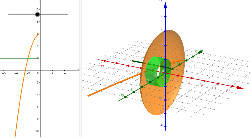
① This example demonstrates how to use GeoGebra's Surface command to revolve a plane curve around an axis, generating a 3D surface of revolution, with a 'slow plotting' feature that reveals the surface's formation step by step. ② Core mathematical concepts include surfaces of revolution, parametric equations, 3D surface construction, and connections to calculus (volume/surface area of solids of revolution). ③ Construction highlights: Based on the summary, the Surface command is used with objects a, f, b, g, c—where f and g likely define the curve or axis, and a, b, c may set parameter ranges or auxiliary controls; adjusting sliders or animation speed enables slow generation for clear visualization. ④ Suitable for high school to undergraduate courses in calculus or solid geometry, ideal for teaching the concept of rotational surfaces and as an introductory 3D modeling exercise.