
Slope Fields of Ordinary Differential Equations
Loading the math board and drawing, please wait…
In collections
UQ-Applied Mathematical Analysis
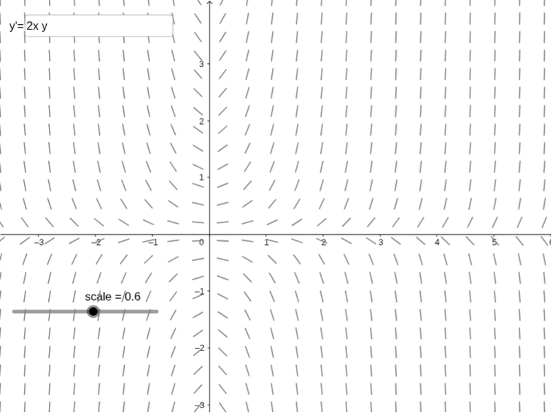
This example demonstrates the slope fields of ordinary differential equations, visually representing the direction of tangents to solutions. Key math concepts include ODEs, slope fields, and solution trajectories. Construction highlights involve commands like SolveODE, Length, First, Element, Segment, SlopeField, and Textfield from GeoGebra. Suitable for high school and above students learning about differential equations and their visual representation.
GeoGebra Commands & Parameters
SolveODE(f, x(A), y(A), xmax, h) → numericalIntegral1SolveODE(f, x(A), y(A), xmin, h) → numericalIntegral2Length(numericalIntegral1) → aFirst(numericalIntegral1, 2000) → list1Element(list1, 1999) → BElement(list1, 2000) → CSegment(B, C) → gSlopeField(f, n, scale) → slopefield1Textfield(f) → InputBox1Textfield(Ax) → InputBox2Textfield(Ay) → InputBox3
AI Drawing Prompt Reference
Draw the slope field of an ordinary differential equation to show the direction of tangents, including solution trajectories. Start by plotting the slope field, then add input boxes for the equation and initial conditions, and finally connect points on the solution trajectory with line segments to form curves.
The prompt above was compiled from the original drawing commands and is for reference only.