
Slope Field by יואב דביר
Loading the math board and drawing, please wait…
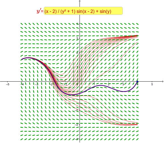
This example illustrates the concept of a slope field and shows the solutions of differential equations. Key mathematical concepts include differential equations and functions. Using GeoGebra commands such as SlopeField, SolveODE, and Sequence, a dynamic slope field can be constructed. Suitable for high school and above students learning calculus and differential equations.
GeoGebra Commands & Parameters
Textfield(f) → inputBox1Textfield(x_{min}) → inputBox2Textfield(x_{max}) → inputBox3Textfield(y_{min}) → inputBox4Textfield(y_{max}) → inputBox5SlopeField(f, 30, 0.5, x_{min}, y_{min}, x_{max}, y_{max}) → SFSolveODE(f, x(A), y(A), x_{max}, 0.01) → SLVFSolveODE(f, x(A), y(A), x_{min}, 0.01) → SLVBSequence(SolveODE[f, 0, t1, x_{max}, 0.01], t1, -2, 2, 0.25) → SLVFLSequence(SolveODE[f, 0, t1, x_{min}, 0.01], t1, -2, 2, 0.25) → SLVBL
AI Drawing Prompt Reference
Draw a slope field by inputting a function expression and setting the minimum and maximum values for x and y. Then, solve the differential equation in the specified range to generate the upper and lower boundary curves of the slope field. Finally, generate multiple upper and lower boundary curves of the slope field in both positive and negative x-axis directions to observe how the solutions of the differential equation change with different initial conditions.
The prompt above was compiled from the original drawing commands and is for reference only.