
Simple Pendulum by Euler Method
Loading the math board and drawing, please wait…
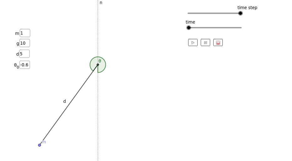
This GeoGebra example demonstrates the motion of a simple pendulum simulated using the Euler numerical method. It visualizes the swinging of a pendulum bob and the evolution of its angle over time. Core mathematical concepts include ordinary differential equations, numerical integration (Euler's method), angular velocity, angular acceleration, torque, and moment of inertia. The construction uses GeoGebra commands such as Textfield, Intersect, Point, Segment, Rotate, Angle, and Line, along with sliders for parameters like gravity, length, mass, and time step. It is suitable for high school or introductory college physics courses to illustrate pendulum dynamics and numerical approximation techniques, as well as for mathematics classes demonstrating solutions to differential equations.
GeoGebra Commands & Parameters
Textfield(m_{1}) → massTextfield(g) → gravityTextfield(d_{1}) → lengthIntersect(xAxis, yAxis) → APoint(Circle[A, d_{1}]) → BSegment(A, B) → fRotate(B, θ_{antes}, A) → mAngle(B, A, m) → θSegment(A, m) → dTextfield(θ_{antes}) → θ_{0}Line(B, A) → n
AI Drawing Prompt Reference
Create a diagram for a simple pendulum simulated with the Euler method: place a pivot point A at the intersection of horizontal and vertical axes, set the pendulum length d, and mark the bob position B using that length from A so that segment AB represents the pendulum rod. Rotate point B around A to an additional starting orientation, forming another segment from A to the rotated position, and mark the angle θ at the pivot between the current bob direction and the rotated reference direction. Include a line through B and A to serve as a direction/angle reference, and add text labels for mass, gravity, length, and the initial angle θ0 to reflect the key parameters used in the numerical simulation.
The prompt above was compiled from the original drawing commands and is for reference only.