
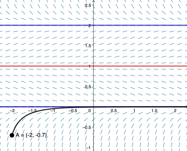
Slope Field and Stable/Unstable Solutions
Loading the math board and drawing, please wait…
In collections
MATH1052-edX
This example demonstrates the geometric representation of differential equation solutions through slope fields. Key mathematical concepts include derivatives, slope fields, and equilibrium points. Construction involves GeoGebra commands SlopeField and SolveODE, using objects yA, button1, A, f, a, F, Sol1, g, h, i. Suitable for high school students learning differential equations intuitively and for university mathematics courses in geometric analysis.
GeoGebra Commands & Parameters
SlopeField(f, 25, 0.7) → FSolveODE(f, x(A), y(A), 10, 0.01) → Sol1
AI Drawing Prompt Reference
Draw a slope field for a differential equation on a coordinate plane, using short line segments to indicate the derivative direction at each point. From a chosen initial point, plot a numerical solution curve that follows the slope field. Include a draggable initial point and an input box for adjusting the equation parameter. The slope field should cover a wide area, and the curve should be smooth and align with the field. Show how solutions change with initial conditions, highlighting stable and unstable equilibrium points.
The prompt above was compiled from the original drawing commands and is for reference only.