
Sinusoidal Transformations
Loading the math board and drawing, please wait…
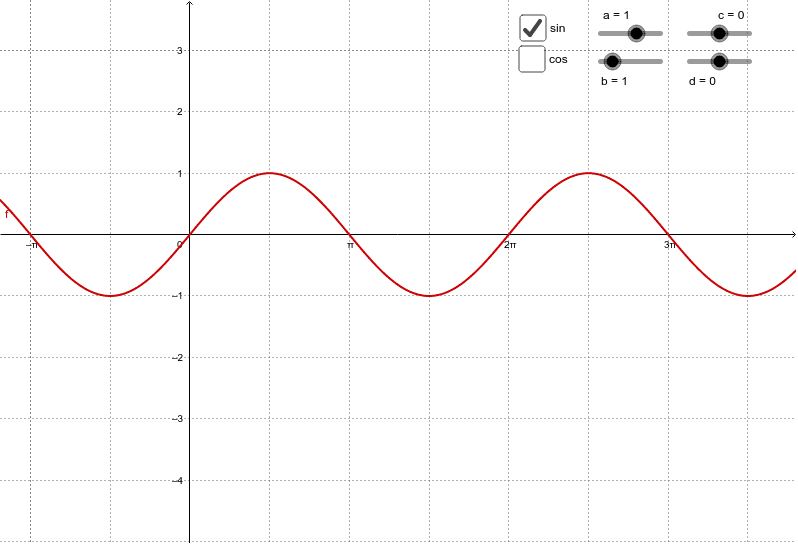
This example demonstrates the graphical transformations of sine and cosine functions. It involves core math concepts like trigonometric functions, function transformations, and coordinate geometry. GeoGebra commands and objects used include a, c, b, c_1, d, text1, f, g, text2, e, h for plotting functions, sliders, and annotations. Suitable for high school mathematics education to understand shifts and scalings in trigonometric graphs.
GeoGebra Commands & Parameters
Numeric a(1.0)Numeric c(0.0015)Numeric b(1.0)c / πNumeric d(0.0)f(x) = (a * sin((b * x) + c)) + dg(x) = (a * cos((b * x) + c)) + dBoolean e(true)Boolean h(false)
AI Drawing Prompt Reference
Draw the graphs of sine and cosine functions to demonstrate transformations caused by parameter changes. Use sliders to control amplitude, frequency, phase shift, and vertical displacement. Set initial amplitude to 1, frequency to 0.0015π, phase shift to 0, and vertical displacement to 0. Display both sine and cosine graphs, and annotate key parameter values.
The prompt above was compiled from the original drawing commands and is for reference only.