
Sine and Cosine Graphs
Loading the math board and drawing, please wait…
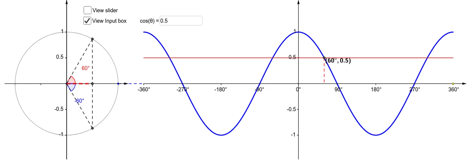
This example demonstrates the plotting of sine and cosine function graphs and their geometric transformations. Key math concepts include trigonometry, geometric transformations, coordinates, and vectors. Construction involves GeoGebra commands like Point, Vector, Circle, Sequence, Segment, Textfield, Intersect, Angle, etc., to build function graphs and geometric elements. Suitable for high school mathematics teaching to understand the properties and applications of trigonometric function graphs and transformations.
GeoGebra Commands & Parameters
Point(Ray[(0, 0), (-1, 0)]) → BVector((x(B), y(Corner[1])), (x(B), y(Corner[4]))) → uVector(B - (1.2, 0), B + (1.2, 0)) → vCircle(B, A) → cVector((0, y(Corner[1])), (0, y(Corner[4]))) → wVector((0 - x(Q), 0), (x(Corner[2]), 0)) → zSequence(Segment[((0.75 * i), 0), ((0.75 * i), -0.025)], i, -4, 4) → list1Sequence(Segment[(0, (0.5 * i) - 1), (-0.025, (0.5 * i) - 1)], i, 0, 4) → list2Sequence(Segment[(x(B), (0.5 * i) - 1), (x(B) - 0.025, (0.5 * i) - 1)], i, 0, 4) → list3Sequence(Segment[B + ((0.5 * i) - 1, 0), B + ((0.5 * i) - 1, -0.025)], i, 0, 4) → list4Segment(A, ((-x(Q)), 0)) → dTextfield(acostheta) → InputBox1Segment(P, (x(P), 0)) → rIntersect(c, j) → C, DSegment(C, G) → mSegment(G, D) → nAngle(A, B, C) → βSegment(B, C) → kSegment(B, D) → lSegment(B, G) → pAngle(A, B, D) → γ