Semicircles in Rectangle: Optimization and Dynamic Loci

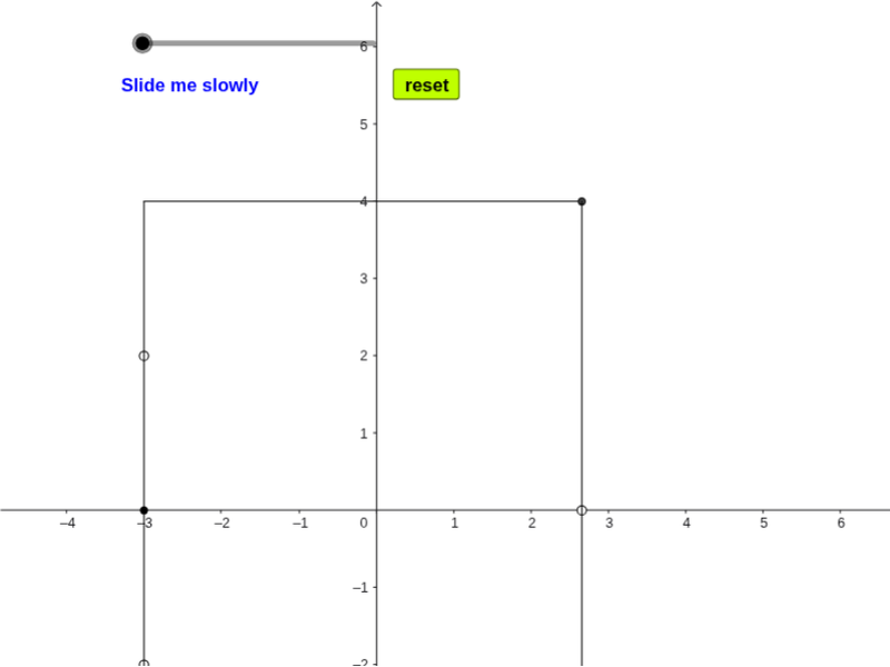
This GeoGebra example dynamically illustrates how semicircles positioned inside a rectangle change in size and position, with a focus on optimizing area or perimeter under geometric constraints. It demonstrates key concepts from coordinate geometry, inequalities, and calculus-based optimization, including tangent conditions and extreme value analysis. Construction uses fundamental GeoGebra commands such as Segment, Circle, Intersect, Semicircle, CircleArc, and CurveCartesian, along with points A, B, C, D, E and other objects to define the rectangle, semicircular arcs, and constraint conditions. The model is suitable for high school mathematics, particularly in optimization and calculus units, and serves as an interactive tool for exploring the interplay between geometric shapes and algebraic constraints.