
Second Order ODE Solver
Loading the math board and drawing, please wait…
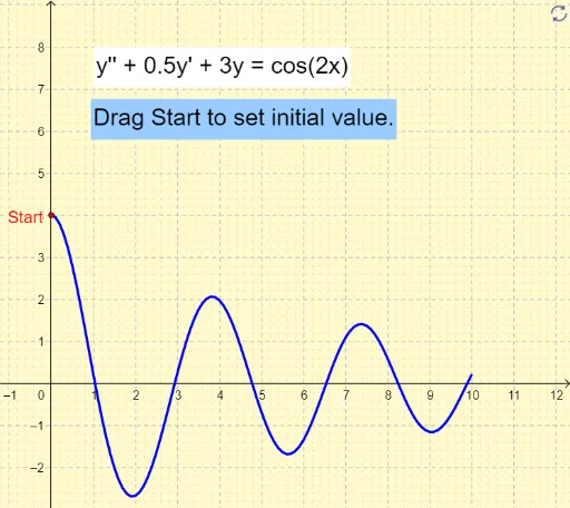
This example demonstrates how to solve second-order ordinary differential equations (ODEs) using GeoGebra's built-in SolveODE command. It involves core mathematical concepts like differential equations, function graphing, and parameter manipulation. Key GeoGebra commands and objects used include Circle, SolveODE, and Textfield, along with variables like Start, d, b, c, f, deltaX, and k for interactive solving and visualization. Suitable for high school students and math enthusiasts exploring ODE solutions and properties.
GeoGebra Commands & Parameters
Circle(Start, 2) → dSolveODE(b, c, f, x(Start), y(Start), k, x(Start) + 10, deltaX) → numeriskIntegral1Textfield(b) → Inmatningsfält1Textfield(c) → Inmatningsfält2Textfield(f) → Inmatningsfält3Textfield(k) → InputBox1Textfield(soln) → InputBox2
AI Drawing Prompt Reference
Create an interactive graph for solving a second-order ordinary differential equation. Draw a reference circle with radius 2 centered at the starting point to mark the initial position. Generate a solution curve starting from that point and extending along the positive x-axis, whose shape is determined by adjustable parameters such as coefficients, initial slope, and step size. Place several input boxes on the interface for adjusting these parameters and displaying the solution result. The layout should clearly show the curve, the reference circle, and the parameter controls, allowing easy observation of how parameter changes affect the solution curve.
The prompt above was compiled from the original drawing commands and is for reference only.