
Second Order Differential Equation - Modified Euler Method - Simple Harmonic Osc
Loading the math board and drawing, please wait…
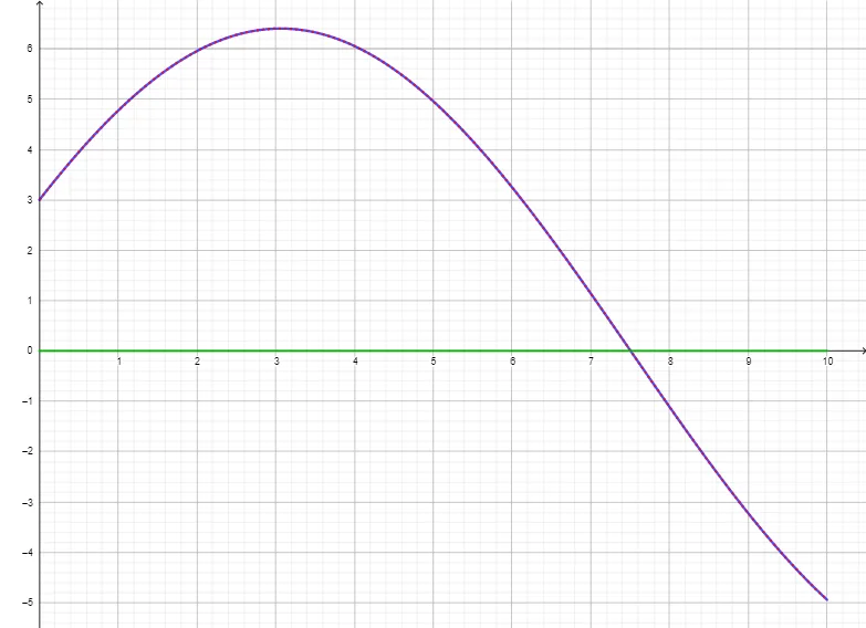
This example demonstrates the solution of second-order differential equations using the modified Euler method to model the motion of simple harmonic oscillators. Key mathematical concepts include second-order differential equations, the modified Euler method, simple harmonic oscillator models, and trigonometric functions. The construction leverages GeoGebra commands such as Sequence, SolveODE, LaTeX, PolyLine, First, Sum, and TableText to generate numerical solutions and trajectory plots, with parameters like k, Z0, Y0, X0, Xf, n, deltaX, and tol controlling the simulation. Suitable for university students in mathematics or physics, and enthusiasts interested in numerical solutions of differential equations.
GeoGebra Commands & Parameters
Sequence((Element[ListaX, i], Element[ListaY, i]), i, 1, Length[ListaX], 1) → LPySolveODE(0, k, 0, X0, Y0, Z0, Xf, deltaX) → numericalIntegral1Sequence((Element[ListaX, i], Element[ListaZ, i]), i, 1, Length[ListaX], 1) → LPy'LaTeX(numericalIntegral1, true, false) → text1PolyLine(LPy) → fFirst(Element[{numericalIntegral1}, 1], Length[Element[{numericalIntegral1}, 1]]) → l1Sequence(abs(Element[ListaY, i] - y(Element[l1, i])), i, 1, Length[ListaY], 1) → LErrorSum(LError) → SErrorPolyLine(Sequence[(Element[ListaX, i], Element[LError, i]), i, 1, Length[ListaY], 1]) → gTableText({LaTeX[SError, true, true]}, {LaTeX[ymax, true, true]}, {LaTeX[ymin, true, true]}) → text2TableText({LaTeX[X0, true, true]}, {LaTeX[Xf, true, true]}, {LaTeX[Y0, true, true]}, {LaTeX[Z0, true, true]}, {LaTeX[deltaX, true, true]}, {LaTeX[n, true, true]}, {LaTeX[tol, true, true]}) → text3