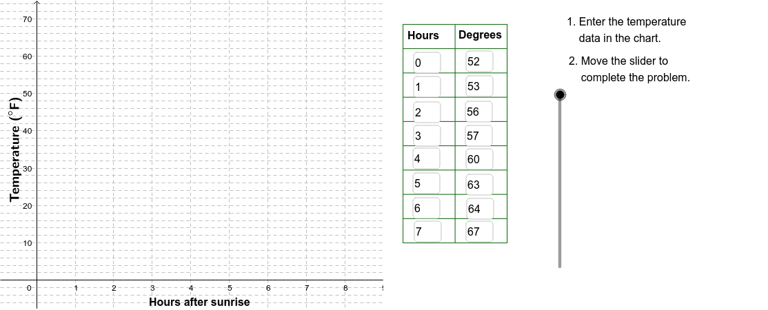
Scatter Plot of Temperature vs. Hours After Sunrise with Linear Fit

This example records the temperature each hour after sunrise on a May morning, plots the data as a scatter plot, and fits a linear function to illustrate the linear relationship between time and temperature. It covers core concepts such as linear equations, linear functions, slope and intercept, as well as the technique of overlaying a function graph on a scatter plot. The construction in GeoGebra employs commands like Corner, Polygon, Textfield, Sequence, Line, and VerticalText, along with objects Corn1–Corn4, Corn2, Corn3, Slid, poly1, etc., to generate point sequences, text labels, and interactive sliders for dynamic visualization. Ideal for middle or high school students learning about functions, data analysis, and introductory GeoGebra usage.