Sampling and Normal Distribution Demo: Dot Plot of Binomial Random Samples

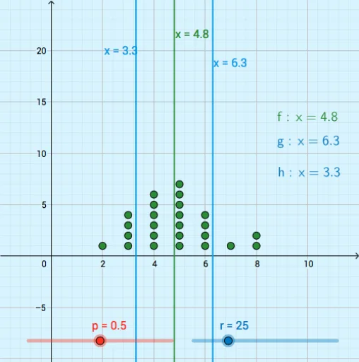
① This example demonstrates how random samples from a binomial distribution are generated and displayed as a dot plot, illustrating the relationship between sampling distributions and the normal approximation. ② Core mathematical concepts include binomial distribution, random sampling, normal distribution, sample statistics, and the foundational idea of the central limit theorem, along with basic operations such as correlation, derivative, addition, and exponentiation used in statistical modeling. ③ Construction highlights: GeoGebra commands RandomBinomial generate random binomial data, Sequence builds sample sequences, DotPlot creates the dot plot, and LaTeX is used for labeling parameters; objects include n (number of trials), p (success probability), a (sample array), r (random value), L_1 and L_2 (data lists), f, h, g (functions or graphical objects), text1-3 (text labels), and coordinate bounds xMin, xMax, yMin, yMax. ④ Suitable for high school or introductory college statistics courses, this helps students grasp sampling variability, conditions for normal approximation, and data visualization techniques, and can serve as an inquiry activity or classroom demonstration tool.