Sample Means Distribution: Repeated Sampling and Histogram

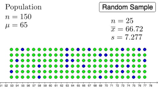
This GeoGebra example dynamically demonstrates the process of repeatedly drawing samples from a population and computing their means, visually illustrating the distribution of sample means. The core mathematical concepts involve sampling distributions, the Central Limit Theorem, and the relationship between sample means and the population mean. Construction highlights include using the DotPlot command to create dot plots, the Sample command to generate random samples, and mean, MeanX, and SampleSDX to calculate sample means and standard deviations. Numerous objects (e.g., A150 to A111) store each sampling result, ultimately forming a histogram of sample means. This resource is suitable for introductory statistics courses at the high school or college level, helping students grasp sampling error and how the distribution of sample means changes with sample size, and can also be used to explore the effect of different sample sizes on the shape of the distribution.