
Rotation vs. Time Simulation by harrytomalley
Loading the math board and drawing, please wait…
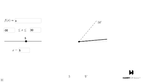
This example demonstrates the dynamic relationship between rotation angle and time, showcasing statistical characteristics of rotation through simulation. Core math concepts include rotation, cube root, statistical characteristics, reflection, solid geometry, Pythagorean theorem, and logarithms. It uses GeoGebra commands like Textfield, Segment, Rotate, Circle, along with sliders and input boxes for dynamic parameter adjustment, making it suitable for high school mathematics education in understanding function graphs, geometric transformations, and data analysis.
GeoGebra Commands & Parameters
Textfield(f) → InputBox1Textfield(a) → InputBox2Textfield(b) → InputBox3Segment(A, B) → gRotate(A, (f(t))°, A) → A'Rotate(B, (f(t))°, A) → B'Segment(A', B') → g'Rotate(A, (h(t) / ((2 * π)) * 360), A) → A'_{1}Rotate(B, ((h(t) / 360 * 2) * π), A) → B'_{1}Segment(A'_{1}, B'_{1}) → g'_{1}Textfield(t) → InputBox4Circle(A, B) → e
AI Drawing Prompt Reference
Draw a dynamic graphic showing the relationship between rotation angle and time. Use a circle and two points A and B, adjust parameters via input boxes to rotate points A and B, forming rotated points A' and B', and then connect A' and B' to form line segment g'. Additionally, adjust parameters to rotate points A and B, forming rotated points A'₁ and B'₁, and then connect A'₁ and B'₁ to form line segment g'₁. Finally, draw a circle e, connecting points A and B.
The prompt above was compiled from the original drawing commands and is for reference only.