
Rhombicosidodecahedron (n=60): Polyhedra with Extreme Distribution of Equivalent
Loading the math board and drawing, please wait…
In collections
₈Polyhedra with extreme distribution of equivalent vertices
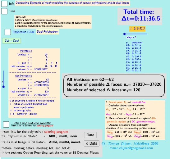
① This example demonstrates the rhombicosidodecahedron, an Archimedean solid with 60 vertices, and explores the extreme distribution of equivalent vertices on a sphere. ② Core mathematical concepts include polyhedral geometry, vertex equivalence, spherical distribution optimization, centroid/barycenter, volume calculation, and linear programming or optimization ideas. ③ Construction highlights: Using GeoGebra commands such as If, Length, Sequence, Sum, Div, Element, TableText, Text, IndexOf, First, Max, the construction builds multiple objects (e.g., Vol, i, A00d, r_d, Volsphere_d, mm-series variables, button3) with parameter n=60 controlling the vertex count, and computes the ratio of sphere volume to polyhedron volume to illustrate the extremal distribution. ④ Suitable for high school and above, useful for solid geometry teaching, mathematical modeling, or computer-aided geometric design, and as a visual case for optimization problems.
GeoGebra Commands & Parameters
If(bu0, A00, A00d) → A00_0Length(A00_0) → nLength(l2) → läl2Sequence(sgn(Determinant[{Element[A00_0, i1] - Element[A00_0, j], Element[A00_0, i2] - Element[A00_0, j], Element[A00_0, i3] - Element[A00_0, j]}]), j, 1, n) → l01Length(A00d) → zzzSum(Zip[(T * F), T, SysTimeAkt1, F, {1, 1000, 60000, 3600000, 86400000}]) → TimeAbs1Sum(Zip[(T * F), T, SysTimeAkt2, F, {1, 1000, 60000, 3600000, 86400000}]) → TimeAbs2Div(TimeRelab, 3600) → HDiv(TimeRelab - (H * 3600), 60) → MElement(ZwZeit, step) → text10TableText({Append["a duration", Last[ZwZeit, Min[10, Length[ZwZeit]]]]}, "v") → text2cLength(A00) → lm1If(Length[Unique[l01 \ {0}]] ≟ 1, 7, -7) → a7Sum(Zip[(T * F), T, SysTimeAkt0, F, {1, 1000, 60000, 3600000, 86400000}]) → TimeAbs0Div(TimeRelab0, 3600) → H0Div(TimeRelab0 - (H0 * 3600), 60) → M0Text("" + (TimeRelab0 - (H0 * 3600) - (M0 * 60))) → S0aText("" + (TimeRelab - (H * 3600) - (M * 60))) → SIndexOf(".", S) → indexIndexOf(".", S0a) → indexaFirst(S, index + 1) → txtSFirst(S0a, indexa + 1) → txtS0aIf(bu0, " ", "d") → txtbuoMax(Length[A00], Length[A00d]) → maxläElement(A00, 24) → m11TableText({{"\underline{Polyhedron}"}, Append["Vertices: n=", {Length[A00]}], Append["r=", {r}], Append["\bar{r}=", {r_m}], Append["k-gon : k=", mm5a], Append["their\; numbers: n_k=", mm7a], Append["Volume: V=", {Vol_r}]}, "hr ") → text7TableText({{"\underline{dual\;Polyhedron}"}, Append["Vertices: n=", {Length[A00d]}], Append["r=", {r_d}], Append[" \bar{r_d}= ", {r_md}], Append["k-gon : k=", mm5ad], Append["their\; numbers: n_k=", mm7ad], Append["Volume: V=", {Vold_r}]}, "hr ") → text20
AI Drawing Prompt Reference
Draw a rhombicosidodecahedron with 60 vertices, an Archimedean solid, to demonstrate the extreme distribution of its vertices on a sphere. Focus on polyhedral geometry, vertex equivalence, spherical distribution optimization, centroid, volume calculation, and optimization concepts. Use parameter n=60 to control vertex count and compute the ratio of sphere volume to polyhedron volume to illustrate the extremal distribution.
The prompt above was compiled from the original drawing commands and is for reference only.