
Biscribed Snub Dodecahedron (n=60): Polyhedra with Extreme Distribution of Equiv
Loading the math board and drawing, please wait…
In collections
₈Polyhedra with extreme distribution of equivalent vertices
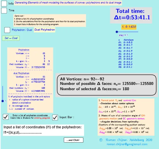
This example demonstrates a biscribed snub dodecahedron with 60 equivalent vertices, belonging to a class of polyhedra that achieve extreme distributions of vertices on a sphere. The core mathematical concepts include vertex equivalence, the property of being both circumscribed and inscribed (biscribed), and optimization methods for distributing vertices uniformly. The construction uses GeoGebra commands such as Sequence, Sum, Div, Element, TableText, and Text to generate vertex coordinates and display data. Key objects include radius variables (r_md, r_d, r_m, r), volume calculations (Vol, Volsphere_d, Vol_r), and auxiliary points (A00, A00d, mm7ad). This example is suitable for high school and above students or math enthusiasts interested in solid geometry, optimization problems, and polyhedron construction.
GeoGebra Commands & Parameters
If(bu0, A00, A00d) → A00_0Length(A00_0) → nLength(l2) → läl2Sequence(sgn(Determinant[{Element[A00_0, i1] - Element[A00_0, j], Element[A00_0, i2] - Element[A00_0, j], Element[A00_0, i3] - Element[A00_0, j]}]), j, 1, n) → l01Length(A00d) → zzzSum(Zip[(T * F), T, SysTimeAkt1, F, {1, 1000, 60000, 3600000, 86400000}]) → TimeAbs1Sum(Zip[(T * F), T, SysTimeAkt2, F, {1, 1000, 60000, 3600000, 86400000}]) → TimeAbs2Div(TimeRelab, 3600) → HDiv(TimeRelab - (H * 3600), 60) → MElement(ZwZeit, step) → text10TableText({{"\underline{Polyhedron}"}, Append["Vertices: n=", {Length[A00]}], Append["r=", {r}], Append["\bar{r}=", {r_m}], Append["k-gon : k=", mm5a], Append["their\; numbers: n_k=", mm7a], Append["Volume: V=", {Vol_r}]}, "hr ") → text7TableText({{"\underline{dual\;Polyhedron}"}, Append["Vertices: n=", {Length[A00d]}], Append["r=", {r_d}], Append[" \bar{r_d}= ", {r_md}], Append["k-gon : k=", mm5ad], Append["their\; numbers: n_k=", mm7ad], Append["Volume: V=", {Vold_r}]}, "hr ") → text20TableText({Append["a duration", Last[ZwZeit, Min[10, Length[ZwZeit]]]]}, "v") → text2cLength(A00) → lm1If(Length[Unique[l01 \ {0}]] ≟ 1, 7, -7) → a7Sum(Zip[(T * F), T, SysTimeAkt0, F, {1, 1000, 60000, 3600000, 86400000}]) → TimeAbs0Div(TimeRelab0, 3600) → H0Div(TimeRelab0 - (H0 * 3600), 60) → M0Text("" + (TimeRelab0 - (H0 * 3600) - (M0 * 60))) → S0aText("" + (TimeRelab - (H * 3600) - (M * 60))) → SIndexOf(".", S) → indexIndexOf(".", S0a) → indexaFirst(S, index + 1) → txtSFirst(S0a, indexa + 1) → txtS0aIf(bu0, " ", "d") → txtbuoMax(Length[A00], Length[A00d]) → maxläElement(A00, 24) → m11
AI Drawing Prompt Reference
Draw a biscribed snub dodecahedron with 60 equivalent vertices, highlighting its extreme vertex distribution. The polyhedron is both circumscribed and inscribed, with vertices uniformly distributed via optimization. Include core radius variables, volume calculations, and auxiliary points, along with key data for the polyhedron and its dual, such as vertex count, radii, polygon types, and volumes.
The prompt above was compiled from the original drawing commands and is for reference only.