
Biscribed Truncated Cuboctahedron, n=48: Polyhedra with Extreme Distribution of
Loading the math board and drawing, please wait…
In collections
₈Polyhedra with extreme distribution of equivalent vertices
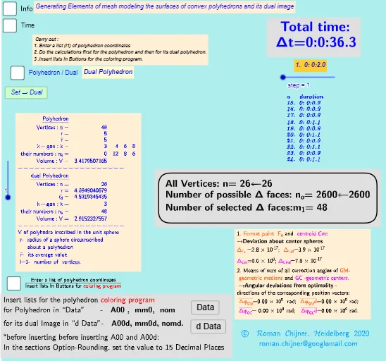
This GeoGebra example demonstrates a biscribed truncated cuboctahedron with 48 equivalent vertices, illustrating a polyhedron with extreme vertex distribution on a sphere. The core mathematical concepts include polyhedral symmetry, vertex equivalence, circumscribed and inscribed spheres (biscribed property), and optimization of vertex placement. The construction uses GeoGebra commands such as Sequence, Sum, Div, Element, If, Length, and TableText to generate and organize vertex coordinates, along with sliders and buttons for interactive exploration. Suitable for high school and university students studying solid geometry, polyhedral constructions, and optimization problems, as well as for mathematical modeling and computational geometry.
GeoGebra Commands & Parameters
If(bu0, A00, A00d) → A00_0Length(A00_0) → nLength(l2) → läl2Sequence(sgn(Determinant[{Element[A00_0, i1] - Element[A00_0, j], Element[A00_0, i2] - Element[A00_0, j], Element[A00_0, i3] - Element[A00_0, j]}]), j, 1, n) → l01Length(A00d) → zzzSum(Zip[(T * F), T, SysTimeAkt1, F, {1, 1000, 60000, 3600000, 86400000}]) → TimeAbs1Sum(Zip[(T * F), T, SysTimeAkt2, F, {1, 1000, 60000, 3600000, 86400000}]) → TimeAbs2Div(TimeRelab, 3600) → HDiv(TimeRelab - (H * 3600), 60) → MElement(ZwZeit, step) → text10TableText({Append["a duration", Last[ZwZeit, Min[10, Length[ZwZeit]]]]}, "v") → text2cLength(A00) → lm1If(Length[Unique[l01 \ {0}]] ≟ 1, 7, -7) → a7Sum(Zip[(T * F), T, SysTimeAkt0, F, {1, 1000, 60000, 3600000, 86400000}]) → TimeAbs0Div(TimeRelab0, 3600) → H0Div(TimeRelab0 - (H0 * 3600), 60) → M0Text("" + (TimeRelab0 - (H0 * 3600) - (M0 * 60))) → S0aText("" + (TimeRelab - (H * 3600) - (M * 60))) → SIndexOf(".", S) → indexIndexOf(".", S0a) → indexaFirst(S, index + 1) → txtSFirst(S0a, indexa + 1) → txtS0aIf(bu0, " ", "d") → txtbuoMax(Length[A00], Length[A00d]) → maxläElement(A00, 24) → m11TableText({{"\underline{Polyhedron}"}, Append["Vertices: n=", {Length[A00]}], Append["r=", {r}], Append["\bar{r}=", {r_m}], Append["k-gon : k=", mm5a], Append["their\; numbers: n_k=", mm7a], Append["Volume: V=", {Vol_r}]}, "hr ") → text7TableText({{"\underline{dual\;Polyhedron}"}, Append["Vertices: n=", {Length[A00d]}], Append["r=", {r_d}], Append[" \bar{r_d}= ", {r_md}], Append["k-gon : k=", mm5ad], Append["their\; numbers: n_k=", mm7ad], Append["Volume: V=", {Vold_r}]}, "hr ") → text20
AI Drawing Prompt Reference
Draw a biscribed truncated cuboctahedron with 48 equivalent vertices, illustrating extreme vertex distribution on a sphere. First, create 48 vertices, then truncate and bisect the cube, ensuring each vertex lies on the sphere, and finally adjust the vertex positions to optimize the distribution.
The prompt above was compiled from the original drawing commands and is for reference only.