
Biscribed Truncated Icosahedron, n=60: Polyhedra with Extreme Distribution of Eq
Loading the math board and drawing, please wait…
In collections
₈Polyhedra with extreme distribution of equivalent vertices
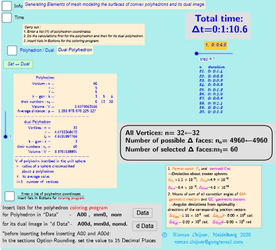
This example demonstrates a biscribed truncated icosahedron with 60 equivalent vertices, belonging to a class of polyhedra that achieve extreme distributions of vertices. The core mathematical concepts involve polyhedral geometry, vertex equivalence, centroid (barycenter), and optimization problems—specifically, finding optimal vertex arrangements under given constraints. The construction uses GeoGebra commands such as Sequence, Sum, If, Length, Element, TableText, and IndexOf, along with objects like sphere volume (Volsphere), volume calculations (Vol), auxiliary points (A00, m01, m02), and sliders for dynamic parameter adjustment. This example is suitable for high school to university-level mathematics, particularly for teaching solid geometry, optimization theory, and computer-assisted geometric construction. It also serves as a tool for exploring symmetry and extreme distributions in polyhedra.
GeoGebra Commands & Parameters
Text("" + p) → txt_pSum(Flatten[Sequence[Append[Sequence[Element[txt_p, i], i, m01(k), m02(k)], " "], k, 1, 5]]) → txtUm1If(bu0, A00, A00d) → A00_0Length(A00_0) → nLength(l2) → läl2Sequence(sgn(Determinant[{Element[A00_0, i1] - Element[A00_0, j], Element[A00_0, i2] - Element[A00_0, j], Element[A00_0, i3] - Element[A00_0, j]}]), j, 1, n) → l01Length(A00d) → zzzSum(Zip[(T * F), T, SysTimeAkt1, F, {1, 1000, 60000, 3600000, 86400000}]) → TimeAbs1Sum(Zip[(T * F), T, SysTimeAkt2, F, {1, 1000, 60000, 3600000, 86400000}]) → TimeAbs2Div(TimeRelab, 3600) → HDiv(TimeRelab - (H * 3600), 60) → MElement(ZwZeit, step) → text10TableText({Append["a duration", Last[ZwZeit, Min[10, Length[ZwZeit]]]]}, "v") → text2cLength(A00) → lm1If(Length[Unique[l01 \ {0}]] ≟ 1, 7, -7) → a7Sum(Zip[(T * F), T, SysTimeAkt0, F, {1, 1000, 60000, 3600000, 86400000}]) → TimeAbs0Div(TimeRelab0, 3600) → H0Div(TimeRelab0 - (H0 * 3600), 60) → M0Text("" + (TimeRelab0 - (H0 * 3600) - (M0 * 60))) → S0aText("" + (TimeRelab - (H * 3600) - (M * 60))) → SIndexOf(".", S) → indexIndexOf(".", S0a) → indexaFirst(S, index + 1) → txtSFirst(S0a, indexa + 1) → txtS0aIf(bu0, " ", "d") → txtbuoMax(Length[A00], Length[A00d]) → maxläElement(A00, 24) → m11TableText({{"\underline{Polyhedron}"}, Append["Vertices: n=", {Length[A00]}], Append["r=", {r}], Append["\bar{r}=", {r_m}], Append["k-gon : k=", mm5a], Append["their\; numbers: n_k=", mm7a], Append["Volume: V=", {Vol_r}], Append["Average\; distance: p=", {txtUm1}]}, "hr ") → text7TableText({{"\underline{dual\;Polyhedron}"}, Append["Vertices: n=", {Length[A00d]}], Append["r=", {r_d}], Append[" \bar{r_d}= ", {r_md}], Append["k-gon : k=", mm5ad], Append["their\; numbers: n_k=", mm7ad], Append["Volume: V=", {Vold_r}]}, "hr ") → text20
AI Drawing Prompt Reference
Draw a biscribed truncated icosahedron with 60 equivalent vertices, belonging to a class of polyhedra with extreme vertex distribution. Include both the primary polyhedron and its dual, displaying key metrics: vertex count, circumradius, mean radius, face edge counts and numbers, volume, and average vertex distance. Construct by first defining the vertex set, then generating faces, and computing centroid and volume. Use sliders for dynamic parameter adjustment, updating numerical tables in real time to explore symmetry and extreme distributions.
The prompt above was compiled from the original drawing commands and is for reference only.