
Review on Gradient and Y-Intercept for Linear Equations
Loading the math board and drawing, please wait…
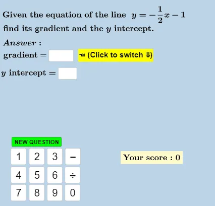
This example demonstrates how students recognize the gradient and y-intercept values of linear equations given in various forms such as y=mx+c, ax+by=c, ax+by+c=0. Core math concepts include linear functions, coordinate geometry, slope, and y-intercept. It is constructed using GeoGebra commands like RandomElement, Random, Expand, If, Textfield, Coefficients, Intersect, Text, GCD; key objects include counter, textanswergradient, textansweryintercept, m, c, etc. Suitable for middle school and above students reviewing linear equation basics.
GeoGebra Commands & Parameters
RandomElement({0, -4, -3, -2, 1, 0, 1, 2, 3, 4, 1 / 2, 1 / 3, 1 / 4, 3 / 4, 1 / 5, 2 / 3, 1 / 5, 2 / 5, 3 / 5, 4 / 5, -1 / 2, -1 / 3, -1 / 4, -3 / 4, -1 / 5, -2 / 3, -1 / 5, -2 / 5, -3 / 5, -4 / 5}) → mRandom(-6, 7) → cExpand(Simplify[(m * x) + c]) → fRandom(-6, 7) → aRandomElement({1, 2, 3, 4, 5, 6}) → bRandom(-7, 9) → c_1If(counter < 5, 1, If[counter < 8, 2, 3]) → typeIf(type ≟ 1, m, If[type ≟ 2, m_d, m_d]) → m_sIf(m_s ≟ m_{ans}, true, false) → answergradientcorrectIf(type ≟ 1, c, c_d) → c_sIf(c_s ≟ c_{ans}, true, false) → answeryinterceptcorrectTextfield(textanswergradient) → InputBox1Textfield(textansweryintercept) → InputBox2Expand(Simplify[(m_s * x) + c_s]) → f_sCoefficients(f) → l1If(m ≟ 0, "", If[abs(m) ≟ 1, If[m > 0, "x", "-x"], If[m > 0, "" + (FractionText[abs(m)]) + "x", "-" + (FractionText[abs(m)]) + "x"]]) → textCoeffXIf(c ≟ 0, "", If[m ≟ 0, If[c > 0, "" + (FractionText[abs(c)]), "-" + (FractionText[abs(c)])], If[c > 0, "+" + (FractionText[abs(c)]), "-" + (FractionText[abs(c)])]]) → textConstIf(c_s ≟ 0, "", If[m_s ≟ 0, If[c_s > 0, "" + (FractionText[abs(c_s)]), "-" + (FractionText[abs(c_s)])], If[c_s > 0, "+" + (FractionText[abs(c_s)]), "-" + (FractionText[abs(c_s)])]]) → textConst_sIf(m_s ≟ 0, "", If[abs(m_s) ≟ 1, If[m_s > 0, "x", "-x"], If[m_s > 0, "" + (FractionText[abs(m_s)]) + "x", "-" + (FractionText[abs(m_s)]) + "x"]]) → textCoeffX_sIntersect(f_s, yAxis) → AIf(f_s(Max[Denominator[m_s], 4]) > 10, (-Max[Denominator[m_s], 4]), Max[Denominator[m_s], 4]) → x_{P}If(x(A) > x(P), Vector[P, (x(A), y(P))], Vector[A, (x(P), y(A))]) → u_{AP}If(x(P) > x(A), Vector[If[y(P) > y(A), Vector[(x(P), y(A)), P], Vector[(x(P), y(A)), P]]], Vector[If[y(P) > y(A), Vector[(x(A), y(P)), A], Vector[(x(A), y(P)), A]]]) → v_{AP}Text(If[m_s < 0, "−", ""]) → textGradientSignText("run = " + (Length[u_{AP}])) → textRunGCD({abs(a), abs(b), abs(c_1)}) → hcf
AI Drawing Prompt Reference
Draw a linear function graph, showing its slope and y-intercept. Randomly generate slope and intercept, convert the linear equation to different forms. Plot the graph in the coordinate system, and label the horizontal and vertical components of the slope with vectors. Display the correct slope and intercept values for students to identify and input.
The prompt above was compiled from the original drawing commands and is for reference only.