
Relationship Between Vocabulary and Reading Frequency
Loading the math board and drawing, please wait…
In collections
UCSS Secondary Math I Unit 4 Lesson 3
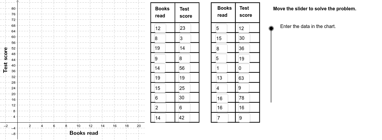
This example analyzes the relationship between a student's vocabulary and their reading frequency, demonstrating basic methods of correlation analysis. Key mathematical concepts include correlation coefficient, scatter plot, and linear regression. GeoGebra commands such as FitLineY and PMCC are used for data fitting and analysis. Suitable for middle school and above students to learn statistical knowledge.
GeoGebra Commands & Parameters
FitLineY(PointList1) → LineFitPMCC(PointList1) → CorCoeffTextfield(A2) → InA2Textfield(A3) → InA3Textfield(A4) → InA4Textfield(A5) → InA5Textfield(A6) → InA6Textfield(A7) → InA7Textfield(A8) → InA8Textfield(A9) → InA9Textfield(A10) → InA10Textfield(A11) → InA11Textfield(A12) → InA12Textfield(A13) → InA13Textfield(A14) → InA14Textfield(A15) → InA15Textfield(A16) → InA16Textfield(A17) → InA17Textfield(A18) → InA18Textfield(A19) → InA19Textfield(A20) → InA20Textfield(A21) → InA21Textfield(B2) → InB2Textfield(B3) → InB3Textfield(B4) → InB4Textfield(B5) → InB5Textfield(B6) → InB6Textfield(B7) → InB7Textfield(B8) → InB8Textfield(B9) → InB9Textfield(B10) → InB10Textfield(B11) → InB11Textfield(B12) → InB12Textfield(B13) → InB13Textfield(B14) → InB14Textfield(B15) → InB15Textfield(B16) → InB16Textfield(B17) → InB17Textfield(B18) → InB18Textfield(B19) → InB19Textfield(B20) → InB20Textfield(B21) → InB21Sequence(Segment[(22, 0 + (7 * i)), (30, 0 + (7 * i))], i, 0, 10) → Linesh1Sequence(Segment[(32, 0 + (7 * i)), (40, 0 + (7 * i))], i, 0, 10) → Linesh2Sequence(Segment[(22 + (4 * i), 0), (22 + (4 * i), 84)], i, 0, 2) → Linesv1Sequence(Segment[(32 + (4 * i), 0), (32 + (4 * i), 84)], i, 0, 2) → Linesv2Segment((22, 84), (30, 84)) → top1Segment((32, 84), (40, 84)) → top2If(LineVisible, "Hide Best Fit Line", "Show Best Fit Line") → LineButtonPolygon((21, y(Corner[1])), Corner[2], Corner[3], (21, y(Corner[4]))) → poly1, a, b, c, dRotateText("Books read", 0) → BottomLegendIf(CorVisible, "Hide Correlation Coefficient", "Show Correlation Coefficient") → CorButtonRotateText("Test score", 90*°) → SideLegend
AI Drawing Prompt Reference
Create a scatter plot with reading frequency on the x-axis and vocabulary size on the y-axis, containing about 20 data points. Add a best-fit line through the points and display the correlation coefficient. Place two data entry tables on the right or below, each with 20 rows for two columns of data. Surround each table with thin grid lines forming rectangular areas, with horizontal and vertical lines creating table cells.
The prompt above was compiled from the original drawing commands and is for reference only.