
Relationship between Histogram and Frequency Polygon
Loading the math board and drawing, please wait…
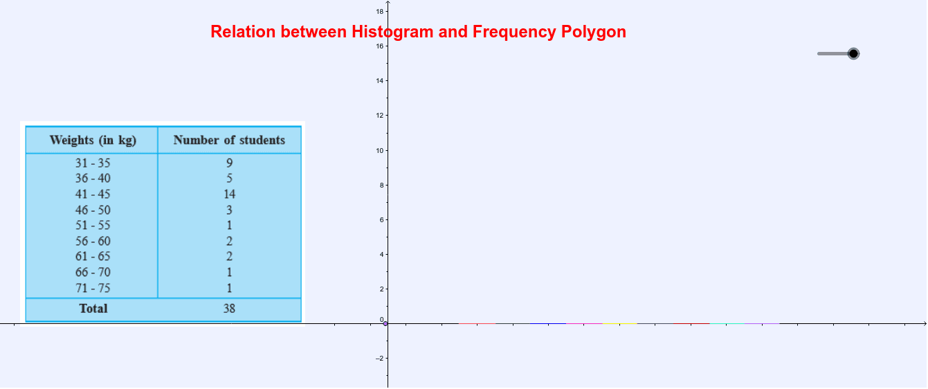
This example demonstrates how histograms and frequency polygons represent the same data distribution in different graphical forms. Key math concepts include data distribution, frequency, and geometric construction. GeoGebra commands/objects used are OrthogonalLine, Point, AttachCopyToView, Polygon, Midpoint, PolyLine, and Line, highlighting the process of transforming histogram data into a polygon. Suitable for high school mathematics education, focusing on statistical chart conversion and comparison.
GeoGebra Commands & Parameters
OrthogonalLine(E_3, xAxis) → f_2Point(f_2) → A_3Point(f_2) → G_2AttachCopyToView(PolyLine[(NaN, NaN), (22.094214551897867, -0.05850817042635832), (22.094214551897867, -0.21819981491899154), (22.11364937414149, -0.33796854828846645), (22.133084196385116, -0.45773728165794136), (22.152519018628738, -0.5775060150274163), (22.152519018628738, -0.7371976595200495), (22.210823485359608, -0.8170434817663661), (22.230258307603233, -0.6573518372737328), (22.249693129846854, -0.5375831039042579), (22.288562774334103, -0.41781437053478304), (22.307997596577724, -0.29804563716530813), (22.32743241882135, -0.13835399267267492), (22.346867241064974, -0.018585259303200024), (22.366302063308595, 0.10118347406627488), (22.38573688555222, 0.22095220743574978), (22.405171707795844, 0.3407209408052247), (22.424606530039465, 0.4604896741746996), (22.44404135228309, 0.5802584075441745), (22.50234581901396, 0.6201813186673328), (22.521780641257582, 0.5004125852978579), (22.521780641257582, 0.3407209408052247), (22.541215463501207, 0.22095220743574978), (22.580085107988452, 0.10118347406627488), (22.599519930232077, -0.05850817042635832), (22.599519930232077, -0.21819981491899154), (22.638389574719323, -0.09843108154951663), (22.638389574719323, 0.06126056294311658), (22.657824396962948, 0.22095220743574978), (22.677259219206572, 0.10118347406627488), (22.696694041450193, -0.05850817042635832), true], 1, (12.84323916393311, -2.4538828378158564), (38.866466148144895, 19.902947391152793), (91.84771873479707, 525.4655286596177), (1430.8477187347983, -34.53447134038237)) → stroke1Point(xAxis) → B_3Point(xAxis) → H_2Point(xAxis) → J_2Point(xAxis) → KPoint(xAxis) → LPoint(xAxis) → MPoint(xAxis) → NPoint(xAxis) → OPoint(xAxis) → PPoint(xAxis) → QPolygon(B_3, R, S, H_2) → poly1, b_1, r, s, hPoint(s) → TPolygon(H_2, T, U, J_2) → poly2, h_1, t, u, jPolygon(J_2, V, W, K) → poly3, j_1, v, w, k_2Point(w) → ZPolygon(K, Z, A_1, L) → poly4, k_1, z_1, a_1, lPoint(a_1) → B_1Polygon(L, B_1, C_1, M) → poly5, l_1, b_2, c_1, m_1Polygon(M, D_1, E_1, N) → poly6, m_2, d_1, e_1, n_1Polygon(N, E_1, F_1, O) → poly7, n_2, e_2, f_1, oPoint(f_1) → G_1Polygon(O, G_1, H_1, P) → poly8, o_1, g_1, h_2, p_1Polygon(H_1, I_1, Q, P) → poly9, h_3, i_1, q_1, p_2Midpoint(r) → J_1Midpoint(v) → K_1Midpoint(t) → L_1Midpoint(z_1) → M_1Midpoint(b_2) → N_1Midpoint(d_1) → O_1Midpoint(e_2) → P_1Midpoint(g_1) → Q_1Midpoint(h_3) → R_1Point(xAxis) → S_1Point(xAxis) → JPolyLine(S_1, J_1, J, L_1, K_1, M_1, N_1, O_1, P_1, Q_1, R_1) → gMidpoint(B_3, H_2) → AMidpoint(H_2, J_2) → BMidpoint(J_2, K) → CMidpoint(K, L) → DMidpoint(L, M) → EMidpoint(M, N) → FMidpoint(N, O) → GMidpoint(O, P) → HMidpoint(P, Q) → IPoint(xAxis) → T_1Point(xAxis) → U_1Line(T_1, U_1) → i