
Rectangular Pyramid Net
Loading the math board and drawing, please wait…
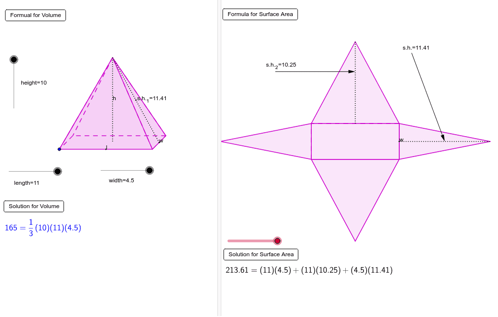
This example demonstrates the construction of a 3D rectangular pyramid model from its net using various geometric transformations and commands. Core math concepts include polygons, solid geometry, vector operations, and geometric transformations. Key GeoGebra commands used are Line, Circle, Intersect, Vector, Translate, Dilate, Midpoint, Polygon, Segment, If, OrthogonalLine, CircleArc, CircumcircleArc, Center, Ray. Suitable for high school students learning solid geometry and spatial visualization skills.
GeoGebra Commands & Parameters
Line(J, K) → hCircle(J, width) → gIntersect(g, h, 1) → MVector(J, M) → wTranslate(A, Vector[w / 2]) → CDilate(I, length, H) → LVector(H, L) → vTranslate(C, v) → DMidpoint(C, D) → Q_1Translate(A, v) → BMidpoint(A, B) → YLine(Y, Q_1) → g_1Midpoint(C, B) → NCircle(Q_1, N) → k_1Intersect(k_1, g_1, 2) → V_1Dilate(F, height, E) → GVector(E, G) → uTranslate(N, u) → OPolygon(A, B, D, C) → P, a, b, d, cPolygon(O, C, D) → Q, d_1, o, c_1Polygon(O, A, C) → R, c_2, o_1, a_1Polygon(O, D, B) → S, b_1, o_2, d_2Polygon(O, A, B) → T, b_2, o_3, a_2Midpoint(B, D) → USegment(O, N) → eSegment(O, U) → fMidpoint(O, U) → WMidpoint(O, N) → VIf(height ≤ 5, C) → ZSegment(Z, O) → iSegment(Z, A) → jLine(N, U) → kIntersect(k, c) → E_1OrthogonalLine(E_1, k) → lOrthogonalLine(U, k) → mCircle(E_1, width / 2) → pIntersect(p, l, 2) → F_1OrthogonalLine(F_1, l) → nIntersect(p, l, 1) → G_1OrthogonalLine(G_1, l) → qIntersect(m, n) → H_1Intersect(m, q) → I_1Midpoint(F_1, H_1) → J_1Midpoint(I_1, G_1) → K_1Line(J_1, K_1) → rCircle(E_1, A1) → sMidpoint(H_1, I_1) → L_1Circle(U, A1) → tIntersect(s, k, 1) → M_1Intersect(t, k, 2) → N_1Circle(J_1, A2) → e_1Circle(K_1, A2) → f_1Intersect(e_1, r, 1) → O_1Intersect(f_1, r, 2) → P_1Vector(O, M_1) → z_1Vector(O, N_1) → i_1Midpoint(Q_1, N) → R_1Midpoint(Y, N) → S_1Circle(S_1, O) → q_1Intersect(q_1, g_1, 1) → T_1Vector(T_1, P_1) → u_1Vector(O, T_1) → w_1Vector(A, G_1) → l_1Vector(B, I_1) → n_1Vector(D, H_1) → r_1Circle(V_1, O) → h_1Vector(C, F_1) → s_1Intersect(h_1, g_1, 2) → U_1Vector(O, U_1) → zVector(U_1, O_1) → j_1CircleArc(S_1, O, T_1) → p_1CircleArc(V_1, U_1, O) → t_1CircumcircleArc(M_1, O, N_1) → e_2Center(e_2) → W_1Translate(O, Vector[(w_1 * m_1)]) → O'Translate(O, Vector[(z_1 * (m_1 - 1))]) → O'_1Translate(O, Vector[(z * (m_1 - 2))]) → O'_2Translate(O, Vector[(i_1 * (m_1 - 3))]) → O'_3Translate(T_1, Vector[(u_1 * (m_1 - 4))]) → Z_1Translate(U_1, Vector[(j_1 * (m_1 - 4))]) → A_2Ray(S_1, O') → f_2Intersect(p_1, f_2, 1) → C_2If(m_1 ≤ 0, O, If[m_1 < 1, C_2, If[m_1 < 4, T_1, If[m_1 < 5, Z_1, P_1]]]) → B_2Ray(W_1, O'_1) → g_2Intersect(e_2, g_2, 1) → D_2If(m_1 ≤ 1, O, If[m_1 < 2, D_2, M_1]) → E_2Ray(W_1, O'_3) → h_2Intersect(e_2, h_2, 1) → F_2If(m_1 ≤ 3, O, If[m_1 < 4, F_2, N_1]) → G_2Ray(V_1, O'_2) → i_2Intersect(t_1, i_2, 1) → H_2If(m_1 ≤ 2, O, If[m_1 < 3, H_2, If[m_1 < 4, U_1, If[m_1 < 5, A_2, O_1]]]) → I_2Translate(A, Vector[(l_1 * (m_1 - 4))]) → A'Translate(B, Vector[(n_1 * (m_1 - 4))]) → B'Translate(D, Vector[(r_1 * (m_1 - 4))]) → D'Translate(C, Vector[(s_1 * (m_1 - 4))]) → C'If(m_1 ≤ 4, A, If[m_1 < 5, A', G_1]) → J_2If(m_1 ≤ 4, C, If[m_1 < 5, C', F_1]) → K_2If(m_1 ≤ 4, D, If[m_1 < 5, D', H_1]) → L_2If(m_1 ≤ 4, B, If[m_1 < 5, B', I_1]) → M_2Polygon(E_2, K_2, J_2) → poly1, j_2, e_3, k_2Polygon(J_2, M_2, B_2) → poly2, b_3, j_3, m_2Polygon(M_2, G_2, L_2) → poly3, l_2, m_3, g_3Polygon(L_2, I_2, K_2) → poly4, k_3, l_3, i_3Polygon(K_2, J_2, M_2, L_2) → poly5, k_4, j_4, m_4, l_4Segment(U, G_2) → n_2Midpoint(U, G_2) → N_2Midpoint(O, U) → O_2Vector(P_2, N_2) → u_2Vector(P_2, O_2) → v_2Segment(N, O) → p_2Midpoint(O, N) → Q_2Segment(A, O) → q_2Segment(B, O) → r_2Segment(D, O) → t_2Segment(C, O) → a_3Segment(U, O) → c_3Midpoint(K_2, L_2) → R_2Segment(R_2, A_2) → d_3Midpoint(Q_2, I_2) → S_2Vector(T_2, S_2) → w_2Segment(J_2, K_2) → f_3