
Reciprocal of a Linear Function
Loading the math board and drawing, please wait…
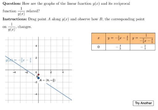
This example demonstrates how to graph and analyze the reciprocal of a linear function, including its asymptotes. Key math concepts involve linear functions, reciprocal functions, asymptotes, and analytical geometry. Construction highlights GeoGebra commands like Polygon, Union, LineToSlopeFormRHS, RemoveUndefined, UnicodeToLetter, LaTeX, Point, Line, Zip, TableText, etc. Suitable for high school students learning function transformations and analytical geometry.
GeoGebra Commands & Parameters
Polygon({(left, top), (right, top), (right, bottom), (left, bottom)}) → viewboxUnion(Sequence[i, i, -5, 5], Zip[xIntercept + A, A, fractions]) → allXvaluesLineToSlopeFormRHS(f) → lineTxtRemoveUndefined(Zip[If[A ≥ minX ∧ A ≤ maxX, A], A, allXvalues]) → useableXvaluesUnicodeToLetter(10007) → xmarkUnicodeToLetter(10003) → cmarkLaTeX("\text{The asymptotes of \(y=\dfrac{1}{g(x)}\) \\occur at the zeros of \(g(x)\). \\The invariant points occur\\when \(y=\pm 1\).}") → fbExplanationLaTeX((((("\text{\textbf{Question: }" * MainInstruc) * "\\\textbf{Instructions: }") * SpecInstruc) * "}")) → allInstrucPoint(Zip[(C, f(C)), C, useableXvalues]) → ALine((xIntercept, 0), yAxis) → vAsymptoteZip((A, f(A)), A, useableXvalues) → useablePointsLaTeX("B") → lblBTableText({titles, dataRow}, "|_c") → dataTable