
Real Component of arctan(z): 3D Surface Visualization
Loading the math board and drawing, please wait…
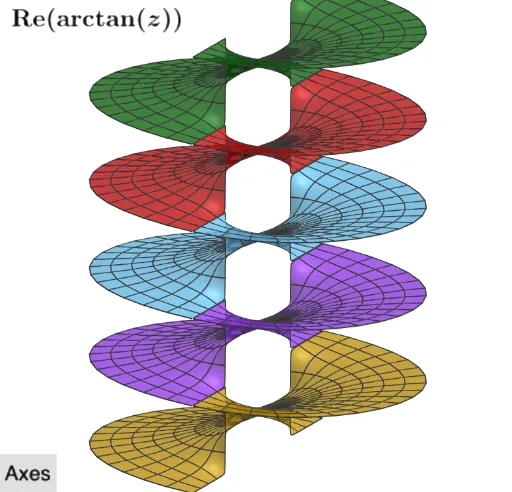
This GeoGebra example visualizes the real part of the complex arctangent function arctan(z) as a 3D surface over the complex plane, revealing the multi-valued nature and branch structure of the inverse tangent. It demonstrates key concepts in complex analysis: multi-valued functions, branch cuts, and the decomposition into real and imaginary parts. The construction uses the Surface command to generate parametric surfaces, with a button and SelectedIndex to switch between different branches (B0 to B4 from ListBranches). Objects like Re, Im, and RSRe control the real/imaginary extraction and surface coloring. Ideal for university-level complex analysis courses or advanced math enthusiasts exploring Riemann surface visualizations and branch behavior.
GeoGebra Commands & Parameters
SelectedIndex(ListBranches) → indexSurface((u * cos(v)), (u * sin(v)), (0 * (1 - t)) + (Re((u * cos(v)), (u * sin(v))) * If[0 ≤ t ≤ 1, t, 1]) + (0 * (2 - t)) + ((π * (0 - 2)) * (1 - t)), u, 0, 2, v, ((-π)) / 2, π / 2 - π / 1000) → B0Surface((u * cos(v)), (u * sin(v)), (0 * (1 - t)) + (Re((u * cos(v)), (u * sin(v))) * If[0 ≤ t ≤ 1, t, 1]) + (0 * (2 - t)) + ((π * (1 - 2)) * (1 - t)), u, 0, 2, v, ((-π)) / 2, π / 2 - π / 1000) → B1Surface((u * cos(v)), (u * sin(v)), (0 * (1 - t)) + (Re((u * cos(v)), (u * sin(v))) * If[0 ≤ t ≤ 1, t, 1]) + (0 * (2 - t)) + (0 * (1 - t)), u, 0, 2, v, ((-π)) / 2, π / 2 - π / 1000) → B2Surface((u * cos(v)), (u * sin(v)), (0 * (1 - t)) + (Re((u * cos(v)), (u * sin(v))) * If[0 ≤ t ≤ 1, t, 1]) + (0 * (2 - t)) + ((π * (3 - 2)) * (1 - t)), u, 0, 2, v, ((-π)) / 2, π / 2 - π / 1000) → B3Surface((u * cos(v)), (u * sin(v)), (0 * (1 - t)) + (Re((u * cos(v)), (u * sin(v))) * If[0 ≤ t ≤ 1, t, 1]) + (0 * (2 - t)) + ((π * (4 - 2)) * (1 - t)), u, 0, 2, v, ((-π)) / 2, π / 2 - π / 1000) → B4Surface((u * cos(v)), (u * sin(v)), (0 * (1 - t)) + (Re((u * cos(v)), (u * sin(v))) * If[0 ≤ t ≤ 1, t, 1]) + (0 * (2 - t)) + ((π * (4 - 2)) * (1 - t)), u, 0, 2, v, π / 2 + π / 1000, (3 * π / 2) - π / 1000) → C4Surface((u * cos(v)), (u * sin(v)), (0 * (1 - t)) + (Re((u * cos(v)), (u * sin(v))) * If[0 ≤ t ≤ 1, t, 1]) + (0 * (2 - t)) + ((π * (0 - 2)) * (1 - t)), u, 0, 2, v, π / 2 + π / 1000, (3 * π / 2) - π / 1000) → C0Surface((u * cos(v)), (u * sin(v)), (0 * (1 - t)) + (Re((u * cos(v)), (u * sin(v))) * If[0 ≤ t ≤ 1, t, 1]) + (0 * (2 - t)) + ((π * (1 - 2)) * (1 - t)), u, 0, 2, v, π / 2 + π / 1000, (3 * π / 2) - π / 1000) → C1Surface((u * cos(v)), (u * sin(v)), (0 * (1 - t)) + (Re((u * cos(v)), (u * sin(v))) * If[0 ≤ t ≤ 1, t, 1]) + (0 * (2 - t)) + (0 * (1 - t)), u, 0, 2, v, π / 2 + π / 1000, (3 * π / 2) - π / 1000) → C2Surface((u * cos(v)), (u * sin(v)), (0 * (1 - t)) + (Re((u * cos(v)), (u * sin(v))) * If[0 ≤ t ≤ 1, t, 1]) + (0 * (2 - t)) + ((π * (3 - 2)) * (1 - t)), u, 0, 2, v, π / 2 + π / 1000, (3 * π / 2) - π / 1000) → C3Surface((u * cos(v)), (u * sin(v)), Re((u * cos(v)), (u * sin(v))), u, 0, 2, v, (-π), π - π / 1000) → RSReSurface((u * cos(v)), (u * sin(v)), Re((u * cos(v)), (u * sin(v))), u, 0, 2, v, π / 2 + π / 1000, (3 * π / 2) - π / 1000) → RSRe2Surface((u * cos(v)), (u * sin(v)), Re((u * cos(v)), (u * sin(v))), u, 0, 2, v, ((-π)) / 2, π / 2 - π / 1000) → RSRe1
AI Drawing Prompt Reference
Create a 3D surface visualizing the real part of the complex arctangent function, showing its multi-valued branch structure. Use polar coordinates with radius from 0 to 2 and angle ranges covering two half-planes (left and right of the imaginary axis). The surface height is given by the real part of arctan, with additional integer multiples of π added to create five parallel branch layers. Leave small angular gaps at the boundaries to reveal branch cuts. Also include a base reference surface without offsets. The result resembles a layered spiral staircase, with distinct colors for each branch, illustrating the Riemann surface of the inverse tangent.
The prompt above was compiled from the original drawing commands and is for reference only.