
Quick-Return Linkage Kinematics: Editable Position, Velocity and Acceleration
Loading the math board and drawing, please wait…
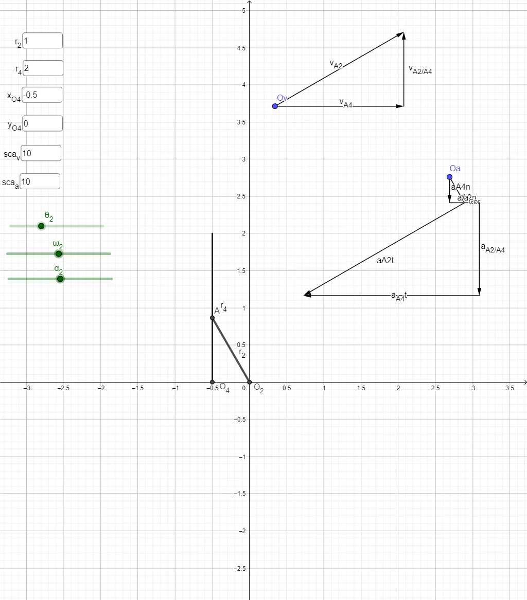
① This example demonstrates the kinematics of a quick-return linkage mechanism, showing position, velocity, and acceleration at any instant with editable parameters. ② Core mathematical concepts include planar linkage kinematics, velocity and acceleration composition for rigid-body motion, vector decomposition into normal and tangential components, and geometric constraint solving for instantaneous positions. ③ Construction highlights: using GeoGebra commands such as Intersect, Circle, Rotate, Vector, Angle, Segment, Point, Line, and OrthogonalLine to build the mechanism; Textfield and InputBox objects allow users to edit crank angle, link lengths, and other parameters; sliders drive the motion, while velocity vectors (vA2, vA4) and acceleration vectors (aA2n, aA2t) are computed and displayed for visualization. ④ Suitable for high school physics or university-level mechanical engineering courses on planar mechanism analysis, this interactive tool helps students intuitively grasp the quick-return characteristic and concepts like instantaneous centers of velocity.
GeoGebra Commands & Parameters
Intersect(xAxis, yAxis) → O_2Circle(O_2, r2) → circO2AIntersect(circO2A, xAxis, 2) → A_{old}Rotate(A_{old}, th2, O_2) → AVector(O_2, A) → pO2ATextfield(xO4) → InputBox1Textfield(r2) → InputBox3Textfield(r4) → InputBox4Textfield(yO4) → yO4editAngle(A_{old}, O_2, A) → th2depSegment(O_2, A) → L2Textfield(scaleV) → InputBox8Textfield(scaleA) → InputBox9Point({xO4, yO4, 0}) → O4Vector(Ov, Ov + (((0, 0, w2) ⊗ pO2A) * scaleV)) → vA2Point({Ov + vA2}) → endvAVector(Oa, Oa + (((0, 0, w2) ⊗ ((0, 0, w2) ⊗ pO2A)) * scaleA)) → aA2nVector(Oa + aA2n, Oa + aA2n + (((0, 0, dw2) ⊗ pO2A) * scaleA)) → aA2tLine(O4, A) → fCircle(O4, r4, xOyPlane) → dIntersect(f, d, 1) → BSegment(O4, B) → L4Vector(O4, A) → pO4AOrthogonalLine(Ov, L4, xOyPlane) → dirVA4Line(endvA, L4) → dirVA2A4Intersect(dirVA4, dirVA2A4) → CVector(Ov, C) → vA4Vector(C, endvA) → vA2A4Vector(Oa, Oa + (((0, 0, w4) ⊗ ((0, 0, w4) ⊗ pO4A)) * scaleA)) → aA4nVector(Oa + aA4n, Oa + aA4n + ((2 * ((0, 0, w4) ⊗ vA2A4)) * scaleA / scaleV)) → aCorPoint({Oa + aA4n + aCor}) → endCorPoint({Oa + aA2n + aA2t}) → endaA2tOrthogonalLine(endaA2t, L4, xOyPlane) → diraA4tLine(endCor, L4) → diraA2A4Intersect(diraA4t, diraA2A4) → DVector(endCor, D) → aA2A4Vector(D, endaA2t) → aA4t
AI Drawing Prompt Reference
Draw a quick-return linkage mechanism showing instantaneous position, velocity, and acceleration. Include two rotation points O2 and O4, and connecting links. Adjust link lengths and angles via input boxes. First, draw point O2, then draw a circle centered at O2, intersecting the x-axis at A_old. Rotate A_old to get A, and draw vector OA. Set parameters via input boxes to draw point O4, and connect O2 and O4 with line segment L2. Calculate and display velocity and acceleration vectors.
The prompt above was compiled from the original drawing commands and is for reference only.