
Quadratic Function Machine: Interactive Visualization of Quadratic Functions wit
Loading the math board and drawing, please wait…
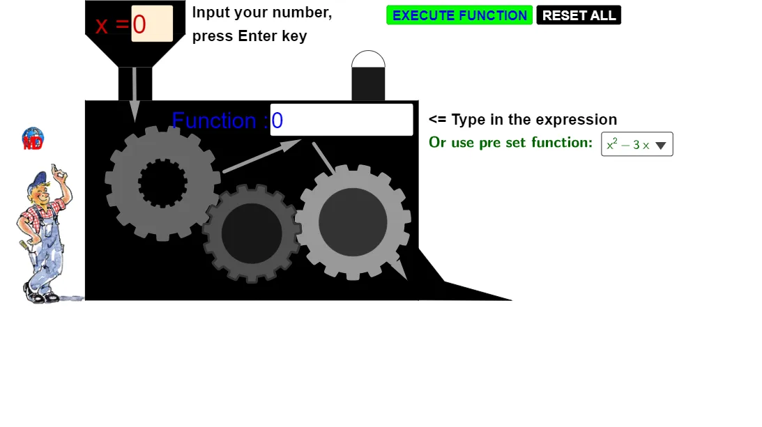
① This interactive 'machine' dynamically demonstrates the graph of a quadratic function and its connections with trigonometric functions, similar triangles, and other geometric elements, allowing users to adjust parameters and observe changes. ② Core mathematical concepts include quadratic functions (parabolas), roots (zeros), trigonometry, similar triangles, dilation (scaling), and intersections. ③ Construction highlights: The example uses GeoGebra commands such as CurveCartesian, Circle, Polygon, Point, Textfield, Vector, Semicircle, Mod, Segment, LaTeX, TextToUnicode, Text, Remove, RemoveUndefined, and Element to build a complex interactive scene with multiple points, polygons, segments, and dynamic text. ④ Suitable for high school or pre-university students learning quadratic functions, trigonometry, and geometric transformations, as well as for teachers to demonstrate the deep connections between functions and geometry in class.
GeoGebra Commands & Parameters
CurveCartesian(x(A) + ((r * (a + (1 / b * tanh((b * sin((n * t) + v)))))) * cos(t + v)), y(A) + ((r * (a + (1 / b * tanh((b * sin((n * t) + v)))))) * sin(t + v)), t, 0, 6.28319) → cCurveCartesian(x(B) + ((R * (a + (1 / b * tanh((b * sin((n * t) - v)))))) * cos(t - v)), y(B) + ((R * (a + (1 / b * tanh((b * sin((n * t) - v)))))) * sin(t - v)), t, 0, 6.28319) → dCircle(B, R + 0.9) → eCircle(A, r + 0.9) → gCircle(A, r + 0.9) → hCurveCartesian(x(A) + ((r * (a + (1 / b * tanh((b * sin((n * t) + v)))))) * cos(t + v)), y(A) + ((r * (a + (1 / b * tanh((b * sin((n * t) + v)))))) * sin(t + v)), t, 0, 6.28319) → iCurveCartesian(x(C) + ((R * (a + (1 / b * tanh((b * sin((n * t) - v)))))) * cos(t - v)), y(C) + ((R * (a + (1 / b * tanh((b * sin((n * t) - v)))))) * sin(t - v)), t, 0, 6.28319) → jCurveCartesian(x(C) + ((r / 2 * (a + (1 / b * tanh((b * sin((n * t) + v)))))) * cos(t + v)), y(C) + ((r / 2 * (a + (1 / b * tanh((b * sin((n * t) + v)))))) * sin(t + v)), t, 0, 6.28319) → oPolygon(D, E, F, G) → poly1, d_1, e_1, f_1, g_1Point(g_1) → HPoint(g_1) → IPolygon(H, I, J, K) → poly2, h_1, i_1, j_1, kPolygon(L, K, J, M) → poly3, l, k_1, j_2, mPoint(f_1) → NPolygon(N, O, P, F) → poly4, n_1, o_1, p, f_2Textfield(s) → ChampTexte1Vector(Q, S) → uTextfield(f) → ChampTexte2Vector(U, V) → wVector(W, Z) → zPolygon(C_1, M, L, D_1) → poly5, c_1, m_1, l_1, d_2Polygon(E_1, F_1, G_1, H_1) → poly6, e_2, f_3, g_2, h_2Semicircle(F_1, G_1) → qMod(v / °, 2) → t_1Semicircle(F_1, G_1) → p_1Segment(A_1, B_1) → a_1LaTeX(f) → textFromFunctionTextToUnicode(textFromFunction) → L_3Text("(" + s + ")") → textFormulaValueTextToUnicode(textFormulaValue) → L_nRemove(Insert[L_n, L_3, IndexOf[120, L_3]], {120}) → L_4Remove(Insert[L_n, L_4, IndexOf[120, L_4]], {120}) → L_5Remove(Insert[L_n, L_5, IndexOf[120, L_5]], {120}) → L_6Remove(Insert[L_n, L_6, IndexOf[120, L_6]], {120}) → L_7Remove(Insert[L_n, L_7, IndexOf[120, L_7]], {120}) → L_8Remove(Insert[L_n, L_8, IndexOf[120, L_8]], {120}) → L_9RemoveUndefined({L_3, L_4, L_5, L_6, L_7, L_8, L_9}) → L_{10}Element(L_{10}, Length[L_{10}]) → L_{11}LaTeX("= " + (UnicodeToText[L_{11}]), true) → textEnumFunction
AI Drawing Prompt Reference
Draw a dynamic quadratic function graph with adjustable parameters, including related trigonometric function graphs. First, draw two dynamic curves, then add two circles, followed by multiple dynamic curves and polygons, and finally add text and vectors to show the relationship between the quadratic function and trigonometric functions.
The prompt above was compiled from the original drawing commands and is for reference only.