
Pythagorean Theorem Animation
Loading the math board and drawing, please wait…
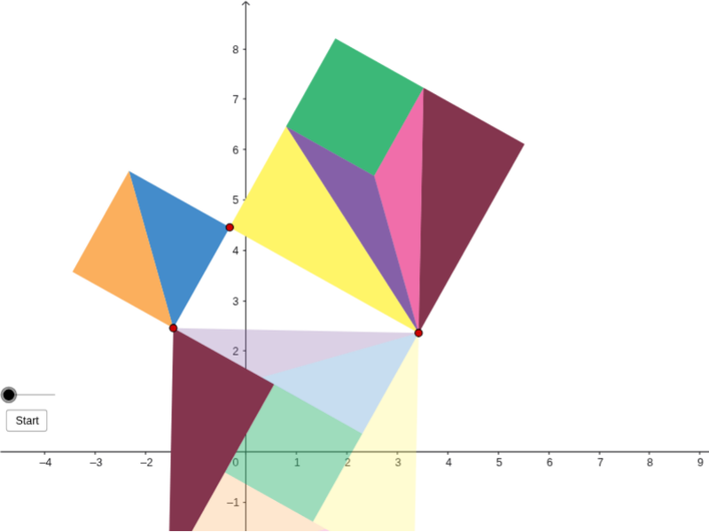
This example demonstrates the Pythagorean Theorem through an animated visualization, clearly illustrating the relationship between the sides of a right triangle. Key mathematical concepts include the Pythagorean Theorem, circles, polygons, rotation, symmetry, and more. The construction utilizes GeoGebra commands such as Semicircle, Intersect, CircleArc, Point, Segment, Mirror, Polygon, OrthogonalLine, Rotate, Midpoint, and If. It is suitable for middle school students and above, as well as for educational purposes in mathematics classes.
GeoGebra Commands & Parameters
Semicircle(A4, A5) → cIntersect(c, LineBisector[A4, A5]) → A,CircleArc(Midpoint[A4, A5], A, A4) → r_1Point(r_1) → A6Segment(A6, A5) → bMirror(A4, b) → A12Polygon(A6, A5, 4) → poly2, c_2, b_1, g, h, A9, A10OrthogonalLine(A12, h) → mSegment(A10, A5) → jIntersect(m, j) → A11Rotate(A6, 90*°, A5) → B8Segment(A4, A6) → aSegment(A5, A4) → dPolygon(A4, A6, 4) → poly1, a_1, c_1, e, f, A7, A8Segment(A4, A7) → iMirror(A12, j) → A13Segment(A5, A12) → k_1Segment(A5, A13) → lSegment(A11, A13) → nSegment(A11, A12) → pPolygon(A5, A4, 4) → poly4, b_2, a_2, k, q, B12, B6Rotate(A11, 90*°, A5) → B7Midpoint(A4, B6) → ORotate(B8, 90*°, O) → B10Rotate(B10, 90*°, O) → B11Rotate(B11, 90*°, O) → B13Rotate(B7, 180*°, O) → B9Segment(B13, B8) → rSegment(B8, B10) → sSegment(B11, B13) → d_1Segment(B11, A4) → e_1Segment(B13, B12) → f_1Segment(B8, B6) → g_1Segment(B10, A5) → h_1Segment(B7, A5) → j_1Segment(B9, B12) → p_1Segment(B10, B11) → q_1Polygon(C4, C5, C6, C7) → poly3, c2, c3, c4, c5Polygon(D4, D5, D6) → poly5, d4, d2, d3Polygon(E4, E5, E6) → poly6, e4, e2, e3Polygon(F4, F5, F6) → poly7, f4, f2, f3Polygon(G4, G5, G6) → poly8, g4, g2, g3Polygon(H4, H5, H6) → poly9, h4, h2, h3Polygon(I4, I5, I6) → poly10, i4, i2, i3If(time < C$2, C4, If[(C$2 ≤ time) ∧ (time < C$3), C4 - (time - C$2) * (C4 - C9) / (C$3 - C$2), C9]) → J4If(time < C$2, C5, If[(C$2 ≤ time) ∧ (time < C$3), C5 - (time - C$2) * (C5 - C10) / (C$3 - C$2), C10]) → J5If(time < C$2, C6, If[(C$2 ≤ time) ∧ (time < C$3), C6 - (time - C$2) * (C6 - C11) / (C$3 - C$2), C11]) → J6If(time < C$2, C7, If[(C$2 ≤ time) ∧ (time < C$3), C7 - (time - C$2) * (C7 - C12) / (C$3 - C$2), C12]) → J7If(time < D$2, D4, If[(D$2 ≤ time) ∧ (time < D$3), D4 - (time - D$2) * (D4 - D9) / (D$3 - D$2), D9]) → K4If(time < D$2, D5, If[(D$2 ≤ time) ∧ (time < D$3), D5 - (time - D$2) * (D5 - D10) / (D$3 - D$2), D10]) → K5If(time < D$2, D6, If[(D$2 ≤ time) ∧ (time < D$3), D6 - (time - D$2) * (D6 - D11) / (D$3 - D$2), D11]) → K6If(time < E$2, E4, If[(E$2 ≤ time) ∧ (time < E$3), E4 - (time - E$2) * (E4 - E9) / (E$3 - E$2), E9]) → L4If(time < E$2, E5, If[(E$2 ≤ time) ∧ (time < E$3), E5 - (time - E$2) * (E5 - E10) / (E$3 - E$2), E10]) → L5If(time < E$2, E6, If[(E$2 ≤ time) ∧ (time < E$3), E6 - (time - E$2) * (E6 - E11) / (E$3 - E$2), E11]) → L6If(time < F$2, F4, If[(F$2 ≤ time) ∧ (time < F$3), F4 - (time - F$2) * (F4 - F9) / (F$3 - F$2), F9]) → M4If(time < F$2, F5, If[(F$2 ≤ time) ∧ (time < F$3), F5 - (time - F$2) * (F5 - F10) / (F$3 - F$2), F10]) → M5If(time < F$2, F6, If[(F$2 ≤ time) ∧ (time < F$3), F6 - (time - F$2) * (F6 - F11) / (F$3 - F$2), F11]) → M6If(time < G$2, G4, If[(G$2 ≤ time) ∧ (time < G$3), G4 - (time - G$2) * (G4 - G9) / (G$3 - G$2), G9]) → N4If(time < G$2, G5, If[(G$2 ≤ time) ∧ (time < G$3), G5 - (time - G$2) * (G5 - G10) / (G$3 - G$2), G10]) → N5If(time < G$2, G6, If[(G$2 ≤ time) ∧ (time < G$3), G6 - (time - G$2) * (G6 - G11) / (G$3 - G$2), G11]) → N6If(time < H$2, H4, If[(H$2 ≤ time) ∧ (time < H$3), H4 - (time - H$2) * (H4 - H9) / (H$3 - H$2), H9]) → O4If(time < H$2, H5, If[(H$2 ≤ time) ∧ (time < H$3), H5 - (time - H$2) * (H5 - H10) / (H$3 - H$2), H10]) → O5If(time < H$2, H6, If[(H$2 ≤ time) ∧ (time < H$3), H6 - (time - H$2) * (H6 - H11) / (H$3 - H$2), H11]) → O6If(time < I$2, I4, If[(I$2 ≤ time) ∧ (time < I$3), I4 - (time - I$2) * (I4 - I9) / (I$3 - I$2), I9]) → P4If(time < I$2, I5, If[(I$2 ≤ time) ∧ (time < I$3), I5 - (time - I$2) * (I5 - I10) / (I$3 - I$2), I10]) → P5If(time < I$2, I6, If[(I$2 ≤ time) ∧ (time < I$3), I6 - (time - I$2) * (I6 - I11) / (I$3 - I$2), I11]) → P6Polygon(J4, J5, J6, J7) → poly11, j4, j5, j6, j7Polygon(K4, K5, K6) → poly12, k6, k4, k5Polygon(L4, L5, L6) → poly13, l6, l4, l5Polygon(M4, M5, M6) → poly14, m6, m4, m5Polygon(N4, N5, N6) → poly15, n6, n4, n5Polygon(O4, O5, O6) → poly16, o6, o4, o5Polygon(P4, P5, P6) → poly17, p6, p4, p5Polygon(C9, C10, C11, C12) → poly18, c9, c10, c11, c12Polygon(D9, D10, D11) → poly19, d11, d9, d10Polygon(E9, E10, E11) → poly20, e11, e9, e10Polygon(F9, F10, F11) → poly21, f11, f9, f10Polygon(G9, G10, G11) → poly22, g11, g9, g10Polygon(H9, H10, H11) → poly23, h11, h9, h10Polygon(I9, I10, I11) → poly24, i11, i9, i10
AI Drawing Prompt Reference
Draw an animated visualization of the Pythagorean theorem, featuring a right triangle with three semicircles and multiple squares. One square's side equals the sum of the triangle's legs, while the other equals the hypotenuse. Show rotation and mirror operations to illustrate the theorem, with dynamic changes in semicircles and squares during the animation, clearly demonstrating the geometric relationships.
The prompt above was compiled from the original drawing commands and is for reference only.