
Pythagorean Comma First Attack
Loading the math board and drawing, please wait…
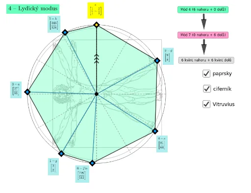
This example demonstrates the manifestation and impact of the Pythagorean comma in geometric figures. It involves core mathematical concepts such as matrices, coordinate geometry, trapezoids, secant lines, and general quadrilaterals. The construction highlights the use of GeoGebra commands/objects like Sequence, Circle, Rotate, Angle, Segment, Intersect, Element, CircleSector, Textfield, Point, Polygon, and Vector. It is suitable for high school and above learners to understand the practical application of complex geometric constructions and mathematical theories.
GeoGebra Commands & Parameters
Sequence((3 / 2)^(k), k, 1, m) → l7Sequence((3 / 2)^(k), k, 1, n) → l5Circle((0, 0), 1) → cSequence((cos((k * π / 6)), sin((k * π / 6))), k, 0, 11, 1) → l1Rotate(B, ((-a) * π / 180), A) → B'Angle(B', A, B) → αSegment(Element[l1, 1], Element[l1, 7]) → fSegment(Element[l1, 2], Element[l1, 8]) → gSegment(Element[l1, 3], Element[l1, 9]) → hSegment(Element[l1, 4], Element[l1, 10]) → iSegment(Element[l1, 5], Element[l1, 11]) → jSegment(Element[l1, 6], Element[l1, 12]) → kSequence((cos(π / 2 + ((2 * π) * log(2, Element[l7, k]))), sin(π / 2 + ((2 * π) * log(2, Element[l7, k])))), k, 1, m, 1) → l6Sequence((cos(π / 2 - ((2 * π) * log(2, Element[l2, k]))), sin(π / 2 - ((2 * π) * log(2, Element[l2, k])))), k, 1, 12, 1) → l3Sequence((cos(π / 2 - ((2 * π) * log(2, Element[l5, k]))), sin(π / 2 - ((2 * π) * log(2, Element[l5, k])))), k, 1, n, 1) → l4Sequence((cos(π / 2 - ((2 * π) * log(2, Element[just5, k]))), sin(π / 2 - ((2 * π) * log(2, Element[just5, k])))), k, 1, 12, 1) → J5Intersect(f, g) → CElement(l4, prvek) → DElement(l6, prvek) → EAngle(D, C, E) → βAngle(D, C, F) → γElement(l4, 2) → HElement(l4, 4) → JElement(l4, 6) → KElement(l4, 1) → LElement(l4, 3) → MElement(l4, 5) → IElement(l6, 5) → NElement(l6, 3) → GElement(l6, 1) → OElement(l6, 4) → PElement(l6, 2) → QCircleSector(C, Element[l4, 1], FF) → qCircleSector(C, Element[l4, 2], Element[l4, 1]) → sCircleSector(C, Element[l4, 3], Element[l4, 2]) → tCircleSector(C, Element[l4, 4], Element[l4, 3]) → c_1CircleSector(C, Element[l4, 5], Element[l4, 4]) → d_1CircleSector(C, Element[l4, 6], Element[l4, 5]) → e_1CircleSector(C, Element[l4, 7], Element[l4, 6]) → f_1CircleSector(C, Element[l4, 8], Element[l4, 7]) → g_1CircleSector(C, Element[l4, 9], Element[l4, 8]) → h_1CircleSector(C, Element[l4, 10], Element[l4, 9]) → k_1CircleSector(C, Element[l4, 11], Element[l4, 10]) → p_1CircleSector(C, Element[l4, 12], Element[l4, 11]) → q_1CircleSector(C, FF, Element[l6, 1]) → r_1CircleSector(C, Element[l6, 1], Element[l6, 2]) → s_1CircleSector(C, Element[l6, 2], Element[l6, 3]) → t_1CircleSector(C, Element[l6, 2], Element[l6, 3]) → c_2CircleSector(C, Element[l6, 3], Element[l6, 4]) → d_2CircleSector(C, Element[l6, 4], Element[l6, 5]) → e_2CircleSector(C, Element[l6, 5], Element[l6, 6]) → f_2CircleSector(C, Element[l6, 6], Element[l6, 7]) → g_2CircleSector(C, Element[l6, 7], Element[l6, 8]) → h_2CircleSector(C, Element[l6, 8], Element[l6, 9]) → k_2CircleSector(C, Element[l6, 9], Element[l6, 10]) → p_2CircleSector(C, Element[l6, 10], Element[l6, 11]) → q_2CircleSector(C, Element[l6, 11], Element[l6, 12]) → r_2CircleSector(C, Element[l4, 12], FF) → s_2CircleSector(C, Element[l4, 7], Element[l6, 5]) → t_2CircleSector(C, Element[l4, 2], Element[l6, 10]) → c_3CircleSector(C, Element[l4, 9], Element[l6, 3]) → d_3CircleSector(C, Element[l4, 4], Element[l6, 8]) → e_3CircleSector(C, Element[l4, 11], Element[l6, 1]) → f_3CircleSector(C, Element[l4, 6], Element[l6, 6]) → g_3CircleSector(C, Element[l4, 1], Element[l6, 11]) → h_3CircleSector(C, Element[l4, 8], Element[l6, 4]) → k_3CircleSector(C, Element[l4, 3], Element[l6, 9]) → p_3CircleSector(C, Element[l4, 10], Element[l6, 2]) → q_3CircleSector(C, Element[l4, 5], Element[l6, 7]) → r_3CircleSector(C, FF, Element[l6, 12]) → s_3Circle(C, v) → t_3Intersect(t_3, i_1, 2) → TRotate(T, (-δ), C) → T'Angle(T', C, T) → εRotate(T', 90°, C) → T''Textfield(δ) → pole1Textfield(m) → pole2Textfield(n) → pole3Segment(QQ, PP) → j_3Point(j_3) → USegment(PP, OO) → i_3Polygon(HH, JJ, OO, LL, MM, II, F) → mnohoúhelník1, hh, jj, oo, ll, mm, ii, f_4Polygon(F, QQ, MM, LL, OO, GG, HH) → mnohoúhelník2, f_5, qq, j_1, l_1, n_1, gg, b_1Polygon(QQ, PP, LL, OO, GG, NN, F) → mnohoúhelník3, i_2, pp, j_2, l_2, m_2, nn, f_6Polygon(OO, LL, PP, QQ, F, HH, GG) → mnohoúhelník4, n_2, a_2, b_2, l_3, f_7, m_3, n_3Polygon(LL, MM, QQ, F, HH, JJ, OO) → mnohoúhelník5, a_3, b_3, g_4, f_8, h_4, i_4, j_4Element(l6, 6) → RPolygon(GG, NN, F, QQ, PP, R, OO) → mnohoúhelník6, k_4, l_4, f_9, m_4, n_4, r_4, p_4Polygon(HH, F, II, MM, LL, KK, JJ) → mnohoúhelník7, q_4, f_{10}, s_4, t_4, a_4, kk, b_4Textfield(δ) → pole4Segment(A, F) → c_4Segment(JJ, A) → d_4Segment(A, HH) → e_4Segment(A, OO) → g_5Segment(A, II) → h_5Segment(A, MM) → i_5Segment(A, LL) → j_5Segment(A, QQ) → k_5Segment(A, GG) → l_5Segment(A, NN) → m_5Segment(A, PP) → n_5Segment(A, KK) → p_5Segment(A, R) → q_5Segment(Q, F) → r_5Vector(S, W) → w_1Vector(Z, A_1) → u_2Segment(Z, S) → s_5Vector(B_1, C_1) → v_2Vector(D_1, E_1) → w_2
AI Drawing Prompt Reference
Draw a circle centered at the origin with radius 1. Place 12 evenly spaced points on the circle and connect them to form a regular hexagon. From one vertex of the hexagon, draw three chords connecting to other vertices on the circle. Based on matrix and coordinate geometry principles, calculate and draw the intersections of these chords with the circle. Then, create multiple sectors from these intersection points. Finally, draw smaller sectors between the larger ones to display the complex pattern formed by these geometric elements.
The prompt above was compiled from the original drawing commands and is for reference only.