
Properties of Quadrilaterals Activity: Doctor Simulator
Loading the math board and drawing, please wait…
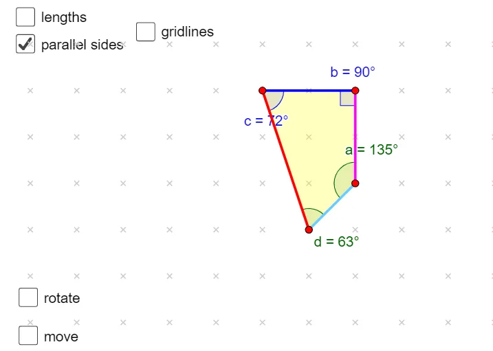
This interactive GeoGebra activity, titled 'Doctor Simulator', dynamically explores the properties of various quadrilaterals including parallelograms, rectangles, rhombi, squares, and trapezoids. It demonstrates how these shapes relate through transformations such as translation and rotation, and highlights concepts of congruence, symmetry, and vector representation. The construction uses commands like Circle, OrthogonalLine, Intersect, Point, Angle, Polygon, Segment, Vector, Rotate, Translate, Midpoint, Ray, CircumcircleArc, and Sequence to build the original quadrilateral poly1 and its transformed copies poly1' and poly1''. Key objects include angle θ, vectors u, v, w, and multiple labeled points and segments, enabling students to visually compare side lengths, angles, and orientation before and after transformations. This activity is ideal for middle or high school geometry classes, supporting inquiry-based learning about quadrilateral classification, congruence, and geometric transformations.
GeoGebra Commands & Parameters
Circle(J, 1) → kOrthogonalLine(J, xAxis) → hIntersect(k, h, 2) → KPoint(k) → LAngle(L, J, K) → θPolygon(A, B, C, D) → poly1, a_{1}, b_{1}, c_{1}, d_{1}Segment(J, K) → eVector(J, L) → uVector(E, J) → vRotate(A, (-θ), I) → A'Rotate(B, (-θ), I) → B'Rotate(C, (-θ), I) → C'Rotate(D, (-θ), I) → D'Polygon(A', B', C', D') → poly1', a', b', c', d'Translate(A', v) → A''Translate(B', v) → B''Translate(C', v) → C''Translate(D', v) → D''Polygon(A'', B'', C'', D'') → poly1'', a'', b'', c'', d''Vector(J, E) → wMidpoint(L, K) → FRay(J, F) → k1Intersect(k, k1) → G,CircumcircleArc(L, G, K) → k2Angle(D'', A'', B'') → αAngle(A'', B'', C'') → βAngle(B'', C'', D'') → γAngle(C'', D'', A'') → δRotate(D'', α, A'') → HAngle(D'', A'', H) → cRotate(A'', α, B'') → MRotate(B'', α, C'') → NRotate(C'', α, D'') → ORotate(A'', β, B'') → PAngle(A'', B'', P) → bRotate(B'', β, C'') → QRotate(C'', β, D'') → RRotate(B'', γ, C'') → SAngle(B'', C'', S) → aRotate(C'', γ, D'') → TRotate(C'', δ, D'') → UAngle(C'', D'', U) → dSegment((x(J) + 0.2, y(J)), (x(J) + 0.4, y(J))) → z11Segment((x(J) + 0.3, y(J) + 0.1), (x(J) + 0.4, y(J))) → z12Segment((x(J) + 0.3, y(J) - 0.1), (x(J) + 0.4, y(J))) → z13Segment((x(J), y(J) + 0.2), (x(J), y(J) + 0.4)) → z21Segment((x(J) - 0.1, y(J) + 0.3), (x(J), y(J) + 0.4)) → z22Segment((x(J) + 0.1, y(J) + 0.3), (x(J), y(J) + 0.4)) → z23Segment((x(J) - 0.2, y(J)), (x(J) - 0.4, y(J))) → z31Segment((x(J) - 0.3, y(J) + 0.1), (x(J) - 0.4, y(J))) → z32Segment((x(J) - 0.3, y(J) - 0.1), (x(J) - 0.4, y(J))) → z33Segment((x(J), y(J) - 0.2), (x(J), y(J) - 0.4)) → z41Segment((x(J) - 0.1, y(J) - 0.3), (x(J), y(J) - 0.4)) → z42Segment((x(J) + 0.1, y(J) - 0.3), (x(J), y(J) - 0.4)) → z43OrthogonalLine(W, yAxis) → fOrthogonalLine(A1, yAxis) → gOrthogonalLine(B1, yAxis) → iOrthogonalLine(C1, yAxis) → jCircle(W, d'') → pIntersect(p, f, 2) → D1Circle(A1, a'') → qCircle(B1, b'') → rIntersect(q, g, 2) → E1Intersect(r, i, 2) → F1Circle(C1, c'') → sIntersect(s, j, 2) → G1Segment(W, D1) → lSegment(A1, E1) → mSegment(B1, F1) → nSegment(C1, G1) → tSegment(E1, D1) → a1Segment(D1, F1) → b1Segment(D1, G1) → c1Segment(E1, F1) → d1Segment(E1, G1) → h1Segment(F1, G1) → i1Vector(Intersect[Circle[Midpoint[d''], 0.125], d'', 2], Intersect[Circle[Midpoint[d''], 0.125], d'', 1]) → u1Vector(Intersect[Circle[Midpoint[b''], 0.12], b'', 1], Intersect[Circle[Midpoint[b''], 0.12], b'', 2]) → u2Vector(Intersect[Circle[Midpoint[a''], 0.2], a'', 1], Midpoint[a'']) → v11Vector(Midpoint[a''], Intersect[Circle[Midpoint[a''], 0.2], a'', 2]) → v12Vector(Midpoint[c''], Intersect[Circle[Midpoint[c''], 0.2], c'', 1]) → v21Vector(Intersect[Circle[Midpoint[c''], 0.2], c'', 2], Midpoint[c'']) → v22Sequence(Sequence[(i', j'), i', -50, 50], j', -50, 50) → list1Sequence(Segment[(j1, -50), (j1, 50)], j1, -50, 50) → list2Sequence(Segment[(-50, j2), (50, j2)], j2, -50, 50) → list3
AI Drawing Prompt Reference
Draw an interactive geometric diagram showing the properties of various quadrilaterals including parallelograms, rectangles, rhombi, and trapezoids. Demonstrate how these shapes relate through translation and rotation, highlighting concepts of congruence, symmetry, and vector representation. Start by drawing a circle and a perpendicular line, finding their intersection point, then construct a quadrilateral using this point. Rotate the quadrilateral around a point by an angle, then translate it to get two new quadrilaterals. Finally, measure the angles of the original and new quadrilaterals, and draw some auxiliary line segments.
The prompt above was compiled from the original drawing commands and is for reference only.