Projectile Motion: Vector and Quadratic Function Dynamic Simulation

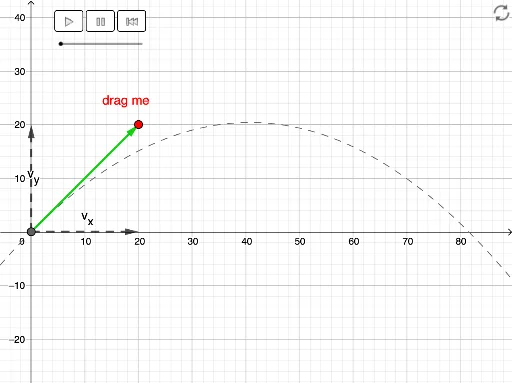
This GeoGebra example dynamically simulates projectile motion, visually demonstrating the parabolic trajectory of an object under gravity. Core mathematical concepts include vector decomposition (horizontal and vertical components of initial velocity), quadratic functions (displacement-time relationships), and how parameter changes affect the path. Construction highlights: the Intersect command finds trajectory-axis intersections, the Vector command constructs velocity vectors, and buttons (button3, button4, button5) along with sliders (t, b, a, d) control time, initial speed, and launch angle for interactive exploration. Suitable for high school physics or mathematics classes teaching projectile motion, vector operations, and quadratic modeling, as well as introductory kinematics in pre-university courses. By dragging parameters, students can observe how range, maximum height, and trajectory shape vary with different initial speeds and launch angles, deepening understanding of motion decomposition and function graphs.