
Visualizing Root-Mean-Squared Rectified Current
Loading the math board and drawing, please wait…
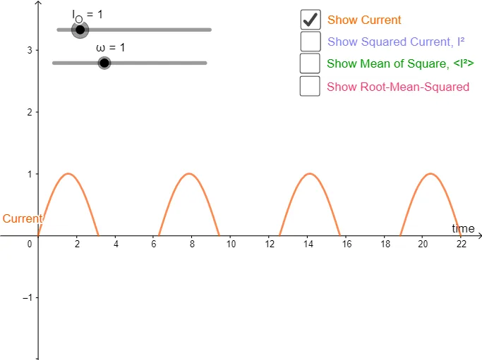
This GeoGebra example demonstrates how to compute and visualize a representative magnitude of a rectified signal by using the root-mean-squared (RMS) idea. It treats the current as a quantity that is “rectified” (nonnegative via taking values appropriately) and then summarizes its behavior through RMS, connecting the numerical statistic to a geometric/graphical representation (e.g., heights in a bar-style view and related geometric constructs). Key concepts include RMS (square-mean then square-root), rectification, and mean-based statistics, with a modeling structure that can be expressed through combinations of intermediate variables and matrix-like organization. From the construction summary, it uses objects such as omega, T, I_O to parameterize the signal, functions f and g to define waveform/model behavior, and additional variables (b, c_1, a, h, p, t, c, d, e, i, j) to build intermediate components and final computed quantities. Text objects (text1) support labeling so the RMS/rectified outcome is clearly identified. Suitable for upper secondary through early university levels, especially for math modeling, graphing, and statistics-to-geometry visualization lessons.
GeoGebra Commands & Parameters
Numeric omega(1)(2 * π / omega)Numeric I_O(1)f(x) = If[x ≥ 0 ∧ sin((omega * x)) ≥ 0, (I_O * sin((omega * x)))]g(x) = f(x)^(2)Boolean b(false)Numeric c_1(0)Integral[g, 0, (2 * π)] / ((2 * π))h(x) = Integral[g(x), 0, (0.5 * T)] / Tp(x) = sqrt(h(x))0Boolean c(true)Boolean d(false)Boolean e(false)Boolean i(false)p(0)
AI Drawing Prompt Reference
In one coordinate plane, visualize a rectified periodic signal using parameters ω and I_O. Define the half-wave rectified waveform f(x): it equals I_O·sin(ωx) when x≥0 and sin(ωx)≥0, and is otherwise 0. Then form g(x)=f(x)^2 to represent the squared (power-like) quantity. Compute an average from g over a cycle by integrating g from 0 to 2π and dividing by 2π, and also build a second normalized mean term h(x) by integrating g(x) over 0 to 0.5T and dividing by T. Finally define p(x)=√h(x) and display the root-mean-squared rectified representative magnitude, with a label indicating “rectified RMS / root-mean-squared of the rectified signal,” highlighting that p is obtained from rectification plus mean and square-root operations (including the value at p(0)).
The prompt above was compiled from the original drawing commands and is for reference only.