
Simulation of Projectile Motion Parabolic Trajectory
Loading the math board and drawing, please wait…
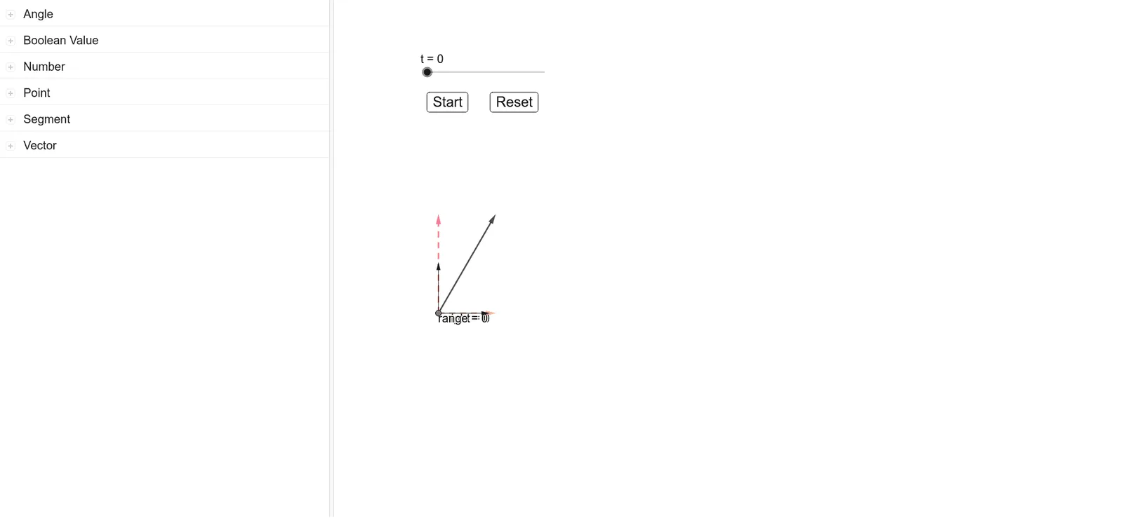
This interactive example demonstrates the parabolic trajectory of a projectile under the influence of gravity. It integrates core mathematical concepts such as quadratic functions, 2D vector decomposition, and parametric equations. The construction utilizes GeoGebra's Vector and Segment commands to visualize velocity and displacement, employing objects like initial velocity (v₀), launch angle (α), gravitational acceleration (a_y), and time (t) to dynamically calculate the position (p_x, p_y), maximum height, and horizontal range. This tool is ideal for high school physics or mathematics students to explore kinematics and the properties of parabolas.
GeoGebra Commands & Parameters
Vector(P, Translate[P, (v_{x}, v_{y})]) → velVector(P, Translate[P, (0, v_{y})]) → vVector(P, Translate[P, (v_{x}, 0)]) → uSegment(P, (p_{x}, y_{0})) → heightSegment((0, 0), (p_{x}, y_{0})) → range
AI Drawing Prompt Reference
Draw a parabolic trajectory of projectile motion. From the origin, show an arrowed vector for initial velocity, decomposed into horizontal and vertical arrowed components. On the curve, mark a moving point, with a vertical dashed line down to the horizontal axis indicating current height, and a horizontal segment from origin to the projection point indicating horizontal displacement. Include coordinate axes, the parabolic path, velocity vector decomposition, and auxiliary lines for height and range, all updating dynamically with parameters.
The prompt above was compiled from the original drawing commands and is for reference only.