Projectile Motion: Parabolic Trajectory with Parameter Decomposition

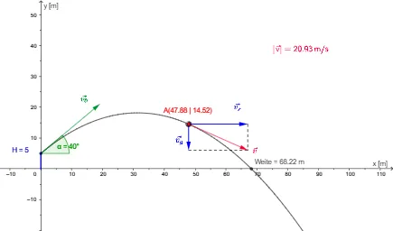
This GeoGebra example demonstrates the complete geometric modeling of oblique projectile motion (schiefer Wurf), showing the parabolic path of an object under gravity. Core mathematical concepts include quadratic functions (parabolic equations), vector decomposition (horizontal and vertical components of initial velocity), angles (launch angle and impact angle), and kinematic relationships between displacement and time. Construction highlights: the Function command defines the parabolic function g, Vector commands create the initial velocity vector v_0 and its components v_x and v_y, Intersect finds the trajectory's ground intersection, Segment draws displacement lines, Root solves for landing time, and Angle labels the launch angle α and impact angle β. Sliders for v_0 and α allow dynamic parameter adjustment. This example is ideal for high school physics or mathematics courses covering projectile motion, quadratic graphs, and vector decomposition, as well as introductory calculus for pre-university students, providing an intuitive visualization of how parameter changes affect trajectory shape.