
Profit and Loss: Interactive Visualization of Business Math
Loading the math board and drawing, please wait…
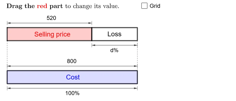
This GeoGebra example provides an interactive visualization of profit and loss scenarios, demonstrating how cost price, selling price, and percentage gain or loss relate dynamically. The core mathematical concepts include percentage calculations, linear relationships, and algebraic equation solving, all embedded in a coordinate geometry framework with points, segments, and vectors. The construction uses commands such as If, Point, Polygon, Sequence, Textfield, Segment, and Vector, along with objects like p, P, b_1, d, a, dtext, m, n, text20, cvalue, b, ctext, c', ntext, dtext', A, B, A0, q, P0, Q, q1, p_1, q_1, g, h, q2, q3, q4, l1-l4, and multiple text boxes and input boxes. It is suitable for middle and high school mathematics classes, especially for teaching percentages, algebraic modeling, and introductory optimization or linear programming. The interactive inputs allow students to change values and immediately see the impact on profit or loss, making abstract business math concepts tangible and engaging.
GeoGebra Commands & Parameters
If(a, "d", ((If[p ∧ x(P) < 10, "-"] * abs(d)) * "")) → dtextIf(c', "c", (n * "")) → ntextPoint(yAxis) → APoint(yAxis) → BIf(x(P) ≤ 10, A + (10, 0), B + (10, 0)) → A0If(x(P) ≤ 10, P, (x(P), y(B))) → P0Polygon(P, Q, (0, y(Q)), (0, y(P))) → q1, p_1, q_1, g, hPolygon({P0, A0, A0 + (0, 1), P0 + (0, 1)}) → q2Polygon({B, B + (10, 0), B + (10, 1), B + (0, 1)}) → q3Polygon({B, B + (10, 0), B + (10, 1), B + (0, 1)}) → q4Sequence(Segment[B + (i, 0), B + (i, 1)], i, 1, 9, 1) → l1Sequence(Sequence[Segment[B + (j + i, 0), B + (j + i, 1)], j, 0, 9, 1], i, 0.1, 0.9, 0.1) → l2Sequence(Segment[A + (i, 0), A + (i, 1)], i, 1, 9, 1) → l3Sequence(Sequence[Segment[A + (j + i, 0), A + (j + i, 1)], j, 0, 9, 1], i, 0.1, 0.9, 0.1) → l4Textfield(n) → InputBox1Textfield(m) → InputBox2If(b, "s", (m * "")) → mtextSegment(If[b_1 ≟ 0, A, A0] + (0, 1.2), If[b_1 ≟ 0, A, A0] + (0, 1.5)) → iSegment(If[b_1 ≟ 0, P, P0] + (0, 1.2), If[b_1 ≟ 0, P, P0] + (0, 1.5)) → jVector(Midpoint[i], Midpoint[j]) → uVector(Midpoint[j], Midpoint[i]) → vSegment(A0 - (0, 0.2), A0 - (0, 0.5)) → kSegment(P0 - (0, 0.2), P0 - (0, 0.5)) → lVector(Midpoint[k], Midpoint[l]) → wVector(Midpoint[l], Midpoint[k]) → eSegment(B + (0, 1.2), B + (0, 1.5)) → fSegment(B + (10, 1.2), B + (10, 1.5)) → rVector(Midpoint[f], Midpoint[r]) → sVector(Midpoint[r], Midpoint[f]) → tSegment(B - (0, 0.2), B - (0, 0.5)) → f_1Segment(B + (10, -0.2), B + (10, -0.5)) → g_1Vector(Midpoint[f_1], Midpoint[g_1]) → u_1Vector(Midpoint[g_1], Midpoint[f_1]) → v_1If(a, "d", If[b, If[b_1 ≟ 0, "s", "x"], "c"]) → text12Sequence(Segment[A + (10 + i, 0), A + (10 + i, 1)], i, 0.1, x(P) - 10, 0.1) → l6Sequence(Segment[A + (10 + i, 0), A + (10 + i, 1)], i, 0, floor(x(P) - 10)) → l5Sequence(Segment[A0 + (i, 0), A0 + (i, 1)], i, 0, floor(x(P0) - 10)) → l7Sequence(Segment[A0 + (i, 0), A0 + (i, 1)], i, 0.1, x(P0) - 10, 0.1) → l8If(p, m - n, abs(n - m)) → cSegment(If[x(P) ≤ 10, A + (10, 0), P], If[x(P) ≤ 10, B + (10, 1), x(P)]) → h_1Segment(A, B + (0, 1)) → i_1Segment(A - (0, 0.2), A - (0, 0.5)) → j_1Segment(P - (0, 0.2), P - (0, 0.5)) → k_1Vector(Midpoint[k_1], Midpoint[j_1]) → w_1Vector(Midpoint[j_1], Midpoint[k_1]) → c_1Segment(A0 + (0, 1.2), A0 + (0, 1.5)) → k'Segment(P0 + (0, 1.2), P0 + (0, 1.5)) → l'Vector(Midpoint[k'], Midpoint[l']) → e_1Vector(Midpoint[l'], Midpoint[k']) → l_1If(p, "Change", If[x(P) < 10, "Loss", If[x(P) > 10, "Profit", ""]]) → change
AI Drawing Prompt Reference
Draw a coordinate system with the x-axis representing cost price and the y-axis representing selling price. Mark cost price point A and selling price point B on the x-axis. Draw two line segments to represent the cost price line and the selling price line based on the input values. Calculate profit or loss using the input values and display the corresponding graph in the coordinate system. Adjust the input values to observe the impact of changes in cost price and selling price on profit or loss.
The prompt above was compiled from the original drawing commands and is for reference only.