
Polynomial Synthetic Division Practice
Loading the math board and drawing, please wait…
In collections
Arithmetic and Algebra
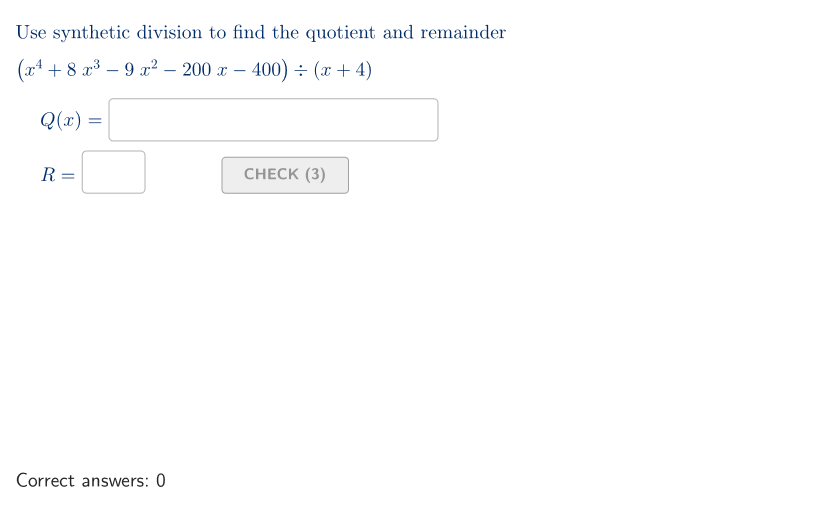
This example demonstrates the complete process of synthetic division (also called Horner's method) for polynomials, helping learners master this essential algebraic technique. Core mathematical concepts include polynomial division, synthetic division, the Remainder Theorem, and the Factor Theorem. The construction generates polynomials with random coefficients, allowing users to input the divisor, quotient, and remainder step by step, with automatic validation. Key GeoGebra commands: Polynomial for constructing polynomials, Div for division operations, Coefficients for extracting polynomial coefficients, If and KeepIf for conditional logic, Textfield for interactive input, and Shuffle for random problem generation. Suitable for upper secondary school and pre-university mathematics courses.
GeoGebra Commands & Parameters
Shuffle({1, 2, 3}) → allCaseNum, {1, 2, 3}Shuffle(Sequence[t, t, -5, 5, 1] \ {0}) → allA, {-4, 1, -3, 5, 2, -1, -5, -2, 3, 4}Shuffle(Sequence[t, t, -5, 5, 1] \ {0}) → allB, {-4, 3, 4, -3, 1, -1, 2, 5, -2, -5}Shuffle(Join[Sequence[Sequence[(j, k), j, -4, 4, 1], k, -4, 4, 1]]) → startGrid, {(4, 3), (-1, -1), (-2, -3), (-2, 0), (3, 2), (0, -3), (0, -2), (4, -3), (-3, 0), (1, -3), (-3, -3), (-1, -3), (1, -1), (-3, 2), (-4, 2), (4, -2), (-2, -1), (4, 4), (0, -4), (-1, 2), (4, 2), (-1, -2), (-3, 4), (1, 3), (-2, 1), (2, 2), (3, -1), (-4, -3), (3, -2), (-2, 4), (-1, 4), (-2, -2), (0, 4), (3, 3), (-1, 1), (-2, 3), (0, -1), (2, 4), (-3, -1), (-1, 0), (0, 0), (-4, -1), (0, 3), (-4, 0), (2, 3), (2, -2), (-4, 1), (-4, -2), (-4, 3), (-4, -4), (-3, 1), (-2, -4), (2, -3), (1, 1), (-1, -4), (2, -4), (1, -4), (3, 0), (4, -1), (3, -4), (-1, 3), (-3, -4), (-4, 4), (-2, 2), (2, -1), (1, 0), (3, 4), (4, 0), (2, 0), (2, 1), (1, -2), (4, -4), (1, 4), (-3, 3), (1, 2), (3, -3), (3, 1), (0, 1), (-3, -2), (4, 1), (0, 2)}Element(allCaseNum, Mod[countQuestion, Length[allCaseNum]] + 1) → caseNumElement(allA, Mod[countQuestion, Length[allA]] + 1) → valAElement(allB, Mod[countQuestion, Length[allB]] + 1) → valBElement(startGrid, Mod[countQuestion, Length[startGrid]] + 1) → V1Shuffle(Sequence[t, t, -5, 5, 1] \ {0}) → allC, {-5, 1, -3, 5, -1, 3, 4, 2, -2, -4}Shuffle(Sequence[t, t, -5, 5, 1] \ {0}) → allD, {5, 1, 2, -5, -1, 4, -3, -2, -4, 3}Shuffle(Sequence[t, t, -5, 5, 1] \ {0}) → allE, {-4, -5, -2, -1, 3, 4, 1, 2, -3, 5}Element(allC, Mod[countQuestion, Length[allC]] + 1) → valCElement(allD, Mod[countQuestion, Length[allD]] + 1) → valDElement(allE, Mod[countQuestion, Length[allE]] + 1) → valEPolynomial(If[caseNum ≟ 1, (((x - valA) * (x - valB)) * (x - valC)), caseNum ≟ 2, ((((x - valA) * (x - valB)) * (x - valC)) * (x - valD)), (((((x - valA) * (x - valB)) * (x - valC)) * (x - valD)) * (x - valE))]) → givenPolyKeepIf(x ≤ 6, DivisorsList[abs(tn)]) → allDivisShuffle({-1, 1}) → allPM, {1, -1}Element(allPM, Mod[countQuestion, Length[allPM]] + 1) → valPMElement(allDivis, Mod[countQuestion, Length[allDivis]] + 1) → divisPolynomial(x + (valPM * divis)) → givenDivisDiv(givenPoly, givenDivis) → givenQuotCoefficients(givenPoly) → allCoeffMod(givenPoly, givenDivis) → givenRemIf(caseNum ≟ 1, 7, caseNum ≟ 2, 9, caseNum ≟ 3, 11) → narrativeChangeTextfield(inputB) → InputBoxBCorner(5) → layoutAppSizeonboardingTextOffset(Corner[onboardingText, 1], Corner[onboardingText, 3], onboardingCase, Corner[1], Corner[3], Corner[5]) → OnboardingTextOffsetTextfield(inputA) → InputBoxATextfield(inputC) → InputBoxCPolygon(P1, Mirror[P1, yAxis], Mirror[P1, (0, 0)], Mirror[P1, xAxis]) → peep, p1, f, g, hShuffle(Sequence[t, t, -6, 6, 1] \ {0, -1, 1}) → allH, {3, -3, -2, 6, -4, 5, 2, 4, -5, -6}If(caseNum ≟ 1, 9, caseNum ≟ 2, 11, 13) → aniMax
AI Drawing Prompt Reference
Create an educational coordinate-plane diagram for practicing polynomial synthetic division (Horner’s method). Generate several randomly chosen integer root locations within the range −5 to 5 excluding 0, and form a given polynomial as a product of factors (x − root) for either three, four, or five such roots depending on the case. On the same graphic, define a corresponding linear divisor in the form x plus a constant determined by a chosen sign times an integer factor, using values consistent with the generated sets. Then display the division outcome by presenting the quotient polynomial and the remainder obtained when dividing the given polynomial by that divisor. Include a clear background grid and an area to show or compare the given polynomial, divisor, quotient, and remainder so the relationships among these objects are visually traceable.
The prompt above was compiled from the original drawing commands and is for reference only.