
Polynomial Inequalities
Loading the math board and drawing, please wait…
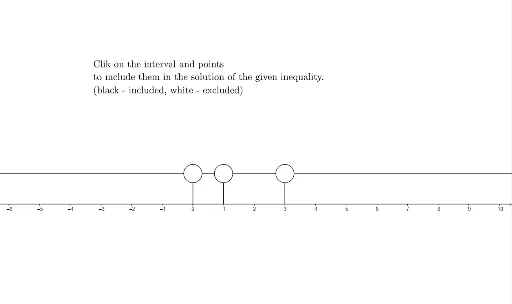
This example demonstrates the graphical representation of polynomial inequalities. Key mathematical concepts include polynomial functions, inequalities, and roots. Using GeoGebra commands such as Element, Polygon, and Circle, one can dynamically explore the roots of polynomials and the solution sets of inequalities. Suitable for high school mathematics education and learning.
GeoGebra Commands & Parameters
Element(Element[problem, prnr], 5) → codePolygon(Corner[1], Corner[2], Corner[3], Corner[4]) → poly1, a, b, c, dElement(Element[problem, prnr], 1) → intextElement(Element[problem, prnr], 2) → x1Element(Element[problem, prnr], 3) → x2Element(Element[problem, prnr], 4) → x3Polygon(Bx0, Bx1, Tx1, Tx0) → int1, bx0, bx1, tx1, tx0Polygon(Bx1, Bx2, Tx2, Tx1) → int2, bx1_1, bx2, tx2, tx1_1Polygon(Bx2, Bx3, Tx3, Tx2) → int3, bx2_1, bx3, tx3, tx2_1Polygon(Bx3, Bx4, Tx4, Tx3) → int4, bx3_1, bx4, tx4, tx3_1Circle(Tx1, 0.3) → eCircle(Tx2, 0.3) → fCircle(Tx3, 0.3) → gLength(problem) → length
AI Drawing Prompt Reference
Draw a graph illustrating polynomial inequalities, showing the function and solution sets. Start by sketching a quadrilateral, then divide the area based on the roots of the inequality, using different colored polygons to represent the solution sets. Add small circles at key points and label the inequality text. The construction order is first draw the base quadrilateral, then divide the regions, and finally add annotations and circles.
The prompt above was compiled from the original drawing commands and is for reference only.