
Polynomial Graphs and Complex Numbers
Loading the math board and drawing, please wait…
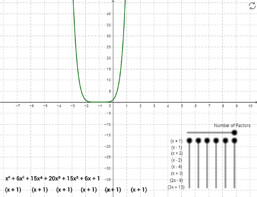
This example demonstrates the graphing of polynomial functions and their relationship with complex numbers. Key math concepts include polynomial functions, complex numbers, parametric curves, secant lines, special points, and symmetry. GeoGebra commands and objects used in the construction include Element, Sequence, setDeg, fix, deg1-6, op, plot, g, points A1-A6, B1, C1-C6, o2-o6, fullPoly, names, and D1-D4. It is suitable for high school mathematics education, helping students understand polynomial properties and complex number applications.
GeoGebra Commands & Parameters
Element(op, A1) → B1Element(op, A2) → B2Element(op, A3) → B3Element(op, A4) → B4Element(op, A5) → B5Element(op, A6) → B6Sequence(Text["(" + (Element[op, i])] + ")", i, 1, Length[op]) → namesElement(names, fix(deg1)) → D1Element(names, fix(deg2)) → D2Element(names, fix(deg3)) → D3Element(names, fix(deg4)) → D4Element(names, fix(deg5)) → D5Element(names, fix(deg6)) → D6Element(op, A7) → B7Element(op, A8) → B8
AI Drawing Prompt Reference
Draw the graphs of six polynomial functions ranging from degree one to six, showing both real and complex roots as points in the complex plane. Include parametric curves that trace the shape of each polynomial, draw secant lines between selected points, and highlight special points such as turning points, inflection points, and points of symmetry. Emphasize the relationship between the polynomial’s coefficients and its complex roots.
The prompt above was compiled from the original drawing commands and is for reference only.