
Normal Distribution Graphs Comparison: Symmetry, Tangents, and Confidence
Loading the math board and drawing, please wait…
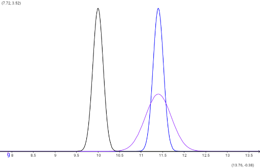
This example demonstrates the comparison of normal distribution curves under varying parameters. Key mathematical concepts include normal distribution, symmetry, tangent lines, percentages, confidence intervals, and function properties. Construction utilizes GeoGebra objects g, f, and SMall to plot curves and analyze statistical features. Suitable for high school or college students learning statistics to visualize distribution characteristics and parameter impacts.
GeoGebra Commands & Parameters
g(x) = (1 / ((0.12 * sqrt((2 * π)))) * exp(((-(x - 11.4)^(2))) / ((2 * 0.12^(2)))))f(x) = (1 / ((0.3 * sqrt((2 * π)))) * ℯ^((-((x - 11.4)^(2) / ((2 * 0.3^(2)))))))SMall(x) = (1 / ((0.12 * sqrt((2 * π)))) * ℯ^((-((x - 10)^(2) / ((2 * 0.12^(2)))))))
AI Drawing Prompt Reference
Draw three normal distribution curves to compare their shapes and positions. The first curve has mean 11.4 and standard deviation 0.12, appearing tall and narrow. The second curve has mean 11.4 and standard deviation 0.3, appearing shorter and wider. The third curve has mean 10 and standard deviation 0.12, shifted to the left. All curves are symmetric about their means, approach the x-axis asymptotically, and have tangent lines at their peaks. The graph should illustrate symmetry, tangent behavior, and the area under the curve for confidence intervals, suitable for statistics education.
The prompt above was compiled from the original drawing commands and is for reference only.