Polar Equation Curve Explorer

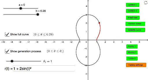
This example demonstrates how to dynamically plot various curves defined by polar equations, with interactive controls to show full or partial curves. The core mathematical concepts include polar-to-Cartesian conversion, parametric equations, function graphing, and curve tracing. Construction highlights: using GeoGebra's CurveCartesian command to convert polar equations into parametric form, employing Textfield input boxes and sliders to adjust parameters r, f, g, a, b, and using buttons to toggle between full and partial curve display, along with text annotations. Suitable for high school or early college students learning polar coordinates, parametric equations, and function graphs, as well as for math labs or exploratory activities to intuitively understand how polar curve shapes change with parameters.